My past experience with glut has been poor. Also, it is not really
part of OpenGL -- various platforms that provide OpenGL do not provide glut.
They all provide "gl" and "glu", the OpenGL utilities library. So the text
uses glut and we will use UIGUI ("oowee gooey", standing for "UI GUI").
It is fine if you want to learn GLUT as well; go right ahead. We will
be learning a lot of "gl" and "glu" in a few weeks.
Generally the operating system and/or window system limit access to the
frame buffer. There is conflict between abstraction and performance. 3D
graphics "accelerator" hardware capabilities are increasingly "higher
level", to where writing to the frame buffer yourself makes less and less
sense.
Homework #0 postulated the use of a primitive for setting an individual
dot (pixel, picture element) on the screen, and the previous lecture
described the frame buffer used to store the contents of the screen in
memory. So, how do we implement DrawPixel() ? The following pseudocode
fragments approximate it for a display WIDTH x HEIGHT whose frame buffer
is an array of bytes for which we have a pointer named fb.
Implementation for real hardware would vary depending e.g. on whether
the processor was "big-endian" or "little-endian", whether a 1-bit
means black or means white, etc.
Another important line algorithm was developed in the 60's and subsequently
refined. Starting from the form F(x,y) = ax + by
There is some cleverness here, to avoid any need for floating
point numbers, which speeds things up greatly, especially on machines that
do not have floating point instructions!
   procedure DrawLine1(x1,y1,x2,y2)
      dx := x2 - x1
      dy := y2 - y1
      d  := 2 * dy - dx
      incrE := 2 * dy
      incrNE := 2 * (dy - dx)
      x := x1
      y := y1
      DrawPoint(x,y)
      while x < x2 do {
         if d <= 0 then {
            d +:= incrE
            x +:= 1
            }
         else {
            d +:= incrNE
            x +:= 1
            y +:= 1
            }
         DrawPoint(x,y)
         }
    end
Midpoint Line Algorithm Example
The best way to get a feel for Bresenham/Midpoint in action is to see it.
Here are the incrE and incrNE, and the value of x, y, and d for the line
segment from (50,50) to (60,63):
incrE 6 incrNE -14
x 50 y 50 d -4
x 51 y 50 d 2
x 52 y 51 d -12
x 53 y 51 d -6
x 54 y 51 d 0
x 55 y 51 d 6
x 56 y 52 d -8
x 57 y 52 d -2
x 58 y 52 d 4
x 59 y 53 d -10
x 60 y 53 d -4
API parameters and graphic contexts
From skimming our text you should notice that
a host of attributes (line width and style, color, etc) are applied
in any given graphic output command. Some API's use separate parameters
for each such "dimension", leading to very large parameter lists. In
the design of the X Window System, this was avoided in order to reduce
network traffic. Instead, resources for drawing attributes are
preallocated on the display server in a large data structure called a
graphics context. The X graphics context is not entirely complete
(e.g. it doesn't include fonts) and other API's subdivide the graphics
context further into specific abstractions such as "pen" and "brush".
Color Indices and Colormaps
So far we have mainly considered monochrome and "true color" frame buffers.
15- and 16-bits per pixel color displays are available that closely
approximate "true color" in behavior. You should learn of at least one very
different method of organizing a frame buffer, commonly used for 4- and
8-bits per pixel color displays. Instead of literally representing
intensity of color, the frame buffer bits on these displays are often used
as subscripts into an array (called a colormap) whose elements are color
intensities.
The "array" may be hardwired to a specific set of colors, or modifiable.
If it is modifiable, the colormap provides a level of indirection that
enables clever (and non-portable) tricks to be played, where modifying
a single array element instantaneously changes the color for many
(possibly hundreds of thousands) pixels.
Circle Drawing
Circles obey the an equation such as
x2 + y2 = R2.
If you can draw a good quarter circle, you
can draw the rest of the circle by symmetry.
If you try to draw a quarter circle by advancing x each step and solving the
equation for y (y == +- sqrt(R2 - x2) from the earlier
equation. But besides being slow, for part of the circle pixels will not
touch because the slope is too steep, similar to the problem we saw drawing
very "steep" lines looping on the x coordinate.
To avoid the discontinuity you can write a loop that steps through
small angular increments and uses sin() and cos() to compute x and y.
- Brute force circle algorithm (based on: y == +- sqrt(R^2 - x^2))
-
How small an angular increment is needed?
our distance is 2 * pi * R pixels worth of drawing;
we need angular increments R small enough to make these adjacent.
1/R radians gives a nice solid circle; angular steps twice as large
still look like a connected, thinner circle.
   procedure DrawCircle0(x,y,R)
      every angle := 0.0 to 2 * &pi by 1.0 / R do {
	 px := x + sin(angle) * R
	 py := y + cos(angle) * R
	 DrawPoint(px,py)
         }
   end
- 8 Way Symmetry
-
Symmetry can speed up and simplify computations. We can do 1/8 as many
calls to sin(), cos(), etc. This code also relies on "translation" of
coordinates from (0,0) to an origin of (x0,y0). Translation is the first
of many coordinate transformations you will see.
   procedure CirclePoints(x0, y0, x, y)
      DrawPoint(x0 + x, y0 + y)
      DrawPoint(x0 + y, y0 + x)
      DrawPoint(x0 + y, y0 - x)
      DrawPoint(x0 + x, y0 - y)
      DrawPoint(x0 - x, y0 - y)
      DrawPoint(x0 - y, y0 - x)
      DrawPoint(x0 - y, y0 + x)
      DrawPoint(x0 - x, y0 + y)
   end
- Mid-point (or Bresenham) circle algorithm
-
Like the mid-point line algorithm, it is possible to do a much more
efficient incremental job of drawing a circle. See Fig 3.14. The
procedure is very similar to the Mid Point line algorithm.
   procedure DrawCircle1(x0,y0,R)
      x := 0
      y := R
      d := 5.0 / 4.0 - R
      CirclePoints(x0, y0, x, y)
      while (y > x) do {
         if d < 0 then {
            d +:= 2.0 * x + 3.0
            }
         else {
	    d +:= 2.0 * (x - y) + 5.0
            y -:= 1
            }
         x +:= 1
	 CirclePoints(x0, y0, x, y)
         }
   end
lecture #4 began here
Restating the Homework Platforms
For doing graphics homeworks, your options are:
- 1. download and install the
necessary graphics libraries and header files to a local machine.
- To run locally, you will have to download an
appropriate libuigui.a and uigui.h in order for your C programs to compile.
In fact, you will have to do this a few times this semester (as libuigui
gets "fleshed out".
In order to use
icon/unicon you would similarly need to download and install unicon from
unicon.org, but that is not required for CS 324.
- 2. ssh into a CS machine.
- For this option, the recommended machine is wormulon.cs.uidaho.edu.
The ssh must be told to support X11 graphics connections.
The command to do this is "ssh -X" from Linux. From Windows
the correct command to do X window forwarding depends on which ssh client
you use, but on the one from ssh.com you would go into the Edit menu, choose
the Settings dialog, click open the Profile Settings, Connection, and
Tunneling tabs, and click the "Tunnel X11 connections" checkbox. From what
I have seen, this option works reasonably well for students at present, and
allows me to update libraries without you having to download them again.
But once we get to assignments where performance matters, being able to run
locally will become a big advantage.
Clarifications on Bresenham/Midpoint Algorithms from Last Lecture
See the book, pages 467-472 for another explanation of Bresenham's
algorithm.
See the
wikipedia article on Bresenham's circle algorithm for a better
description of that algorithm, using integer-only operations. An example
program circ.icn is worth playing with.
Raster Operations
Our hardware lesson for today is yet another nuance of frame buffer
manipulation. Consider the frame buffer as an array of bits in memory.
When you are "drawing" on the frame buffer, you are writing some new bits
out to that memory. You have the option of just replacing and discarding
what used to be there, but there are other possibilities that involve
combining the new value with the old. Each bit of the current
contents could be combined using AND, OR, and NOT with corresponding bits
being output. These different boolean combinations of current frame
buffer with new output pixel values are called raster operations.
The most interesting raster operation is probably XOR. It has the property
that XOR'ing a pixel value a second time restores the pixel to its former
contents, giving you an easy "undo" for simple graphics. On monochrome
displays XOR works like a champion, but on color displays it is less useful,
because the act of XOR'ing in a pixel value may produce seemingly random
or indistinct changes, especially on color index displays where the bits
being changed are not color intensities. If a color display uses mostly
a foreground color being drawn on a background color, drawing the XOR
of the foreground and background colors in XOR mode works pretty much
the way regular XOR does on monochrome displays.
Major Concepts from Hill/Kelley Chapter 2
Note: chapter 2 contains a bunch of introduction to OpenGL, covering
various functions, mainly from the gl and glut libraries. In some
sense it is profoundly overcomplicated. Absorb what you can,
and ask what you want, while we use our much simpler library for awhile.
- absolute vs. relative coordinates
- compare DrawPoint(x1,y1,x2,y3) with DrawTo(xNew, yNew), where
xOld and yOld are an implicit "current drawing position".
- window coordinates vs. screen coordinates
- pixel coordinates are generally relative to a current window...
- normalized coordinates
- going from (0.0,0.0) to (1.0,1.0) gives device independence
- aspect ratio
- width/height matters. For example drawings in normalized coordinates
may look funny if computed with different aspect ratio than displayed.
- event-driven programming
- give up on your ownership of control flow, for most of the semester,
you write function bodies that get called when the graphics system
feels like it. In UIGUI this is "optional" but in OpenGL and most
GUI class libraries it is mandatory. Creates problems for novices
(need to "think backwards"; can't use program counter to remember
where you are any more). Remember where you are by using a state
machine (state variable(s)). For your functions to get called by
the graphics system, you have to tell the system about them (register).
lecture #5 began here
Check it out; it provides some useful information on our current labs.
An Overview of UIGUI's Graphics Primitives
Note: uigui.h and libuigui.a were updated last night for all
platforms to add the DrawLine() primitive. More to come!
Icon/Unicon 2D facilities consist of around 45 functions in total.
There is one new data type (Window) which has around 30 attributes,
manipulated using strings. Most graphics API's introduce a few hundred
functions and several dozens of new typedefs and struct types that you
must memorize.
UIGUI will eventually have around 90 if each of the 45 requires two C versions.
These facilities are mainly described in Chapters 3 and 4 of the Icon
Graphics Book. Here are some of my favorite functions you should start
with. The main differences between Icon/Unicon and UIGUI: the C functions
are not able to take an optional initial parameter, and do not yet support
multiple primitives with a single call. This is less useful in C than in
Icon anyhow, since C does not have an "apply" operator.
An initial "working set" of UIGUI primitives will consist of just under
half of the whole 2D API:
- WOpen(), WClose()
- Open and close the default window. Stickiness around the issue of
initial attributes.
- WAttrib(), Fg(), Bg()
- Get/set an attribute. Fg() and Bg() are common special cases
- DrawPoint(), DrawLine()
- We have seen these by now.
- {Draw,Fill}{Arc,Circle,Polygon,Rectangle}
- 8 functions for other common 2D primitives. In Icon; forthcoming in UIGUI.
Built-ins in underlying Xlib/Win32/hardware.
- DrawCurve()
- A smooth curve algorithm with nice properties. In Icon; forthcoming in UIGUI. Implemented in software.
- Event()
- read a keyboard OR mouse event. In another lecture or two we will
get around to discussing the extra information available about an
event beyond its return value "code". Especially: mouse location.
- Pixel()
- Read the contents of a screen pixel (in Icon: a rectangular region).
In Icon; forthcoming in UIGUI.
Region Filling
Suppose you want to fill in a circle or rectangle you've just drawn using
one of the last few algorithms we've discussed? Starting from a point
inside the object to be filled, one can examine pixels, and set all of
them to a new color until one hits the border color of the object.
The border that defines a region may be 4-connected or 8-connected.
4-connected regions do not consider diagonals to be adjacent; 8-connected
regions do. The following algorithms demonstrate brute force filling.
The foreground color is presumed to be set to "new".
# for interior-defined regions. old must not == new
procedure floodfill_4(x,y,old,new)
   if Pixel(x,y,1,1) === old then {
      DrawPoint(x,y)
      floodfill_4(x,y-1,old,new)
      floodfill_4(x,y+1,old,new)
      floodfill_4(x-1,y,old,new)
      floodfill_4(x+1,y,old,new)
      }
end
For the example we started with (filling in one of our circles) only slightly
more is needed:
# for boundary-defined regions.  the new color may be == to the boundary
procedure boundaryfill_4(x, y, boundary, new)
   p := Pixel(x,y,1,1) # read pixel
   if p ~== boundary & p ~== new then {
      DrawPoint(x,y)
      boundaryfill_4(x,y-1,boundary,new)
      boundaryfill_4(x,y+1,boundary,new)
      boundaryfill_4(x-1,y,boundary,new)
      boundaryfill_4(x+1,y,boundary,new)
      }
end
The main limitation of these brute-force approaches is that the recursion is
deep, slow, and heavily redundant. One way to do better is to fill all
adjacent pixels along one dimension with a loop, and recurse only on the
other dimension.
More reading the frame buffer with Pixel()
If you try one of the fill algorithms above, they do genuinely recurse
crazily enough to get stack overflows. Another reason they are sooo slow
is because of the X11 window system architecture, which does not support
reading the frame buffer as efficiently as writing to it; in particular, to
ask for the contents of a window in general you must send a network message
and wait for a reply.
Pixel(x,y,w,h) asks for all the pixels in a rectangular region with a
single network transaction, which will be must faster than reading each
pixel individually. In general, client-side "image" structures are not
interchangeable with server-side "pixmap" and "window" structures, but
this is an unfortunate limitation of their design.
How, how do you store a local (client-side) copy of a window in order
to work with it efficiently? There are many ways you can represent an
image, but we will start with a couple of brute force representations
using lists of lists and tables of tables.
lecture #6 began here
Where we are at in the Course
I've given you reading assignments in chapter 2, but about half of that
chapter is gross, low-level OpenGL details that I want to you to skim over,
and half are important and useful ideas and principles I want you to "get".
This week we will plow on into Chapter 3.
Q&A
Q: What is the default window size under UIGUI?
A: 80 columns, 12 rows, in the system default "fixed" font.
Q: function watt() doesn't work, what up?
A: watt() supported most context attributes out of the box, but needed
some more code to catch canvas attributes such as size=. Code has been
added; new library build will come shortly.
Parameterizing Figures
Textbook example 2.3.3 illustrates an important concept, which is to
code generic graphics and the apply them in different situations using
different parameters to modify details. A 5-vertex house shape with a
4-vertex chimney are "parameterized" with a translation (peak.x,peak.y)
and a scale (given as a width and height). This is a precursor of
things to come (transformations, Hill chapter 5). If you push this
"add flexibility to my graphics code" theme farther you end up with
"write generic code that reads all the data from a file", another theme
that Hill promotes. Anyhow, let's do a house shape using normalized
coordinates and apply translation and scaling, as an exercise.
Convex Polygons
While we're discussing region filling, I mentioned that the 3D facilities
(in OpenGL) support FillPolygon, but the polygons must be convex. See
your Hill textbook, page 69 for a discussion of this and a definition of
convex polygons. We'll come back to the topic in the 2nd half of the course.
Golden Rectangle
The Hill text page 86-87 has a discussion of the "golden rectangle".
Following the golden ratio, 1.618033989... Note that the HDTV aspect
ratio of 16:9 is closer to the golden ratio than the old 4:3 aspect
ratio, but it sure is wider/skinnier than the real thing.
Faster Fills
To speedup the fill algorithm, one can
- Eliminate recursion, replace it with list operations and loops
- Reduce the number of redundant checks on each pixel
- Think in terms of line segments instead of individual pixels when possible.
# nonrecursive boundary fill.  the new color may be == to the boundary
procedure nr_boundaryfill_4(x, y, boundary, new)
   L := [x, y]
   while *L > 0 do {
      x := pop(L)
      y := pop(L)
      p := Pixel(x,y,1,1) # read pixel
      if p ~== boundary & p ~== new then {
         DrawPoint(x,y)
	 put(L, x, y-1)
	 put(L, x, y+1)
	 put(L, x-1, y)
	 put(L, x+1, y)
         }
      }
end
Backing Store and Expose Events
Using UIGUI we operate under the illusion that each on-screen canvas is
a chunk of the frame buffer that we control as long as our program requires
it. In reality, window systems are sharing and coordinating use of the
frame buffer much as operating systems schedule the CPU. In particular,
moving, resizing, overlapping, minimizing and maximizing windows all
point out the fact that an application doesn't have exclusive or
continuous access to the frame buffer.
Under these various circumstances, window systems may discard part or all
of an application's screen contents, and ask the application to redraw
the needed portion of the screen later, when needed. A window system
tells an application to redraw its screen by sending it an "expose" or
"paint" event. Some applications just maintain a data structure containing
the screen contents and redraw the screen by traversing this data structure;
this is the raster graphics analog of the old "display list" systems used
in early vector graphics hardware. But clients are complicated
unnecessarily if they have to remember what they have already done.
The obvious thing to do, and the thing that was done almost immediately,
was to add to the window system the ability to store screen contents in
an off-screen bitmap called a backing store, and let it do its own redrawing.
Unfortunately, evil software monopolists at AT&T Bell Labs such as Rob Pike
patented this technique, despite not having invented it, and despite its
being obvious. This leaves us in the position of violating
someone's patent whenever we use, for example, the X Window System.
Contexts and Cloning
Last lecture we introduced (via whiteboard) the concepts of graphics
contexts, and cloning the context. This is an expanded treatment of
that.
With certain limits, you can have multiple contexts associated with a
canvas, or can use a context on multiple canvases. Clone(w) creates
an additional context on window w. Attributes in a context include:
- colors: fg, bg, reverse, drawop, gamma
- text: font, fheight, ...
- drawing: fillstyle, linestyle, linewidth, pattern
- clipping: clipx, clipy, clipw, cliph
- translation: dx, dy
In contrast, canvas attributes:
- window: label, image, canvas, pos, posx, posy
- size: resize, size, height, width, rows, columns
- icon: iconpos, iconlabel, iconimage
- text: echo, cursor, x, y, row, col
- pointer: pointer, pointerx, pointery, pointerrow, pointercol
- screen: display, depth, displayheight, displaywidth
lecture #7 began here
Announcements
- Class canceled; homework due date extended
-
Offhand, it looks like I will be unable to teach on Wednesday 9/10.
HW#2 is due Friday.
- MW next week you have guest lectures
-
My excellent doctoral student Jafar will tell you a bit about our
graphics-related research. He is a more bona-fide OpenGL guru than
I, so check out his cool stuff.
lecture #8 began here
Check Out HW#3
"World Window" and "Viewport"
These Hill Ch. 3 concepts are important. The world window specifies
what portion of a scene is to be rendered. Things outside the world
window must be removed at some point from the calculations of what to draw.
The viewport defines where on the physical display this world window is to
appear. Rectangles are usually used for both of these, and if their
aspect ratios do not match, interesting stretching may occur.
"World coordinates" are coordinates defined using application domain
units. Graphics application writers usually find it far easier to
write their programs using world-coordinates. Within the "world",
the graphics application presents one or more rectangle views, denoted
"world-coordinate windows", that thanks to translation, scaling, and
rotation, might show the entire world, or might focus on a very tiny
area in great detail.
A second set of transformations is applied to the graphics primitives to
get to the "physical coordinates", or "viewport" of whatever hardware is
rendering the graphics. The viewport's physical coordinates might refer
to screen coordinates, printer device coordinates, or the window system's
window coordinates.
If the world coordinates and the physical coordinates do not have the
same height-width aspect ratio, the window-to-viewport transformation
distorts the image. Avoiding distortion requires either that the
"world-coordinate window" rectangles match the viewport rectangles' shapes,
or that part of the viewport pixels go unused and the image is smaller.
Fonts
"xlsfonts" reports 5315 fonts on the Linux system in my office.
Windows systems vary even more than X11 systems, since applications
often install their own fonts.
Fonts have: height, width, ascent, descent, baseline. Font portability
is one of the major remaining "issues" in Icon's graphics facilities.
There are four "portable font names": mono, typewriter, sans, serif,
but unless/until these become bit-for-bit identical, programs that use
text require care and/or adjustment in order to achieve portability.
You can "fish for a font" with something like:
Font(("Frutiger"|"Univers"|"Helvetica"|"sans") || ",14")
Proportional width fonts may be substantially more useful, but require
substantially more computation to use well than do fixed width fonts.
TextWidth(s) tells how many pixels wide string s is in a window's current
font. Here is an example that performs text justification.
procedure justify(allwords, x, y, w)
   sofar := 0
   thisline := []
   while word := pop(allwords) do {
      if sofar + TextWidth(word) + (*thisline+1) * TextWidth(" ") > w then {
         setline(x, y, thisline, (w - sofar) / real(*thisline))
         thisline := []
         sofar := 0
	 y +:= WAttrib("fheight")
         }
      }
end
procedure setline(x,y,L,spacing)
   while word := pop(L) do {
      DrawString(x,y,word)
      x +:= TextWidth(s) + spacing
      }
end
Smooth Curves
DrawCurve(x1,y1,...,xN,yN) draws a smooth curve. If first and last points
are the same, the curve is closed and is smooth around this boundary point.
The algorithm used in UIGUI comes from [Barry/Goldman 88] in the SIGGRAPH 88
conference proceedings. Let's see how much we can derive from principles.
How do you draw smooth curves? You can approximate them with
"polylines" and if you make the segments small enough, you will
have the desired smoothness property. But how do you calculate
the polylines for a smooth curve?
- brute force
- You can just represent the curve with every
point on it, or with very tiny polylines. This method is memory
intensive and makes manipulating the curve untenably tedious.
The remaining options represent the curve with mathematical function(s)
that approximate the curve.
- explicit functions y=f(x)
- does not handle curves which "double back"
- implicit equations f(x,y)=0
- hard to write equations for parts of curves, hard to sew multiple curves
together smoothly
- parametric equations x=x(t) y=y(t)
- avoids problems with slopes; complex curves are sewn together from
simpler ones; usually cubic polynomials are sufficient for 3D.
Sewing together curves is a big issue: the "slope" (endpoint tangent vectors
are used to track these) of both curves must be equal at the join point.
Splines
In the real world, a spline is a metal strip that can be bent into various
shapes by pulling specific points on the strip in some direction with some
amount of force. The mathematical equivalent is a continuous cubic
polynomial that passes through a set of control points. There are lots of
different splines with interesting mathematics behind them. Catmull-Rom
splines are one popular family of splines, with the property that the
slopes as the curve passes through each point will be parallel to the
surrounding points (Figure 11.32). Icon's DrawCurve() function uses
the Catmull-Rom splines, specifically the algorithm cited in CG as
[BARR88b]: Barry, Phillip J., and Goldman, Ronald N. (1988).
A Recursive Evaluation Algorithm for a class of Catmull-Rom Splines.
SIGGRAPH'88 conference, published in Computer Graphics 22(4), 199-204.
Smooth Curves - an algorithm
You stitch together the whole curve by doing one chunk at a time; that is,
each outer step of the algorithm draws the spline between two adjacent points
of the supplied vertices. Within that outer step, there are guts to setup the
matrices for this spline segment, and a loop to plot the points.
Since we are drawing a smooth curve piecewise, to do the curve
segment between pi and pi+1 you need four
points actually; you need the points pi-1 and pi+2
in order to do the job. The algorithm will step through the i's
starting with i=4 (3 if you were C language going 0..3 as your first 4 points),
and counting i that way as the point after the two points whose
segment we are drawing, the steps will actually render the curve between
pi-2 and pi-1.
The data type used in the Icon implementation is a record Point with
fields x and y. Under X11 you could use XPoint and under MS Windows,
POINT would denote the same thing (duh).
record Point(x,y)
There
are interesting questions at the endpoints! The algorithm
always needs some pi-1 and pi+2 so at the endpoints
one must supply them somehow.
Icon, Unicon, and UIGUI use the following rule:
 if p1 == pN then
    add pN-1 before p1 and p2 after pN.
 else
    duplicate p1 and pN at their respective ends.
Consequently, I have added this to the front of the gencurve() procedure
for the lecture notes.
# generate a smooth curve between a list of points
procedure gencurve(p)

   if (p[1].x == p[-1].x) & (p[1].y == p[-1].y) then { # close
      push(p, copy(p[-2]))
      put(p, copy(p[2]))
      }
   else { # replicate
      push(p,copy(p[1]))
      put(p,copy(p[-1]))
   }
Now to draw every segment between pi-2 and pi-1.
This is a "for" loop:
every i := 4 to *p do {
Build the coefficients ax, ay, bx and b_y, using:
(note: b_y not "by", because by is an Icon reserved word).
This part is "magic": you have to lookup MCR
and GiBs in the journal article yourself.
                           _              _   _    _
 i                 i    1 | -1   3  -3   1 | | Pi-3 |
Q (t) = T * M   * G   = - |  2  -5   4  -1 | | Pi-2 |
             CR    Bs   2 | -1   0   1   0 | | Pi-1 |
                          |_ 0   2   0   0_| |_Pi  _|
Given the magic, it is clear how the ax/ay/bx/b_y are calculated:
      ax := - p[i-3].x + 3 * p[i-2].x - 3 * p[i-1].x + p[i].x
      ay := - p[i-3].y + 3 * p[i-2].y - 3 * p[i-1].y + p[i].y
      bx := 2 * p[i-3].x - 5 * p[i-2].x + 4 * p[i-1].x - p[i].x
      b_y := 2 * p[i-3].y - 5 * p[i-2].y + 4 * p[i-1].y - p[i].y
Calculate the forward differences for the (parametric) function using
parametric intervals. These used to be intervals of size 0.1 along the
total curve; that wasn't smooth enough for large curves, so they were
expanded to max(x or y axis difference). This is a Bug! It is not always
big enough! What is the correct number to use??
      steps := max(abs(p[i-1].x - p[i-2].x), abs(p[i-1].y - p[i-2].y)) + 10
      stepsize := 1.0 / steps
      stepsize2 := stepsize * stepsize
      stepsize3 := stepsize * stepsize2
      thepoints := [ ]
From here on out as far as Dr. J is concerned this is
basic calculus and can be understood by analogy to physics.
dx/dy are velocities, d2x/d2y are accelerations, and d3x/d3y
are the changes in those accelerations... The 0.5's and the
applications of cubes and squares are from the "magic matrix"...
      x := p[i-2].x
      y := p[i-2].y
      put(thepoints, x, y)
      dx := (stepsize3*0.5)*ax + (stepsize2*0.5)*bx +
	   (stepsize*0.5)*(p[i-1].x-p[i-3].x)
      dy := (stepsize3*0.5)*ay + (stepsize2*0.5)*b_y +
	   (stepsize*0.5)*(p[i-1].y-p[i-3].y)
      d2x := (stepsize3*3) * ax + stepsize2 * bx
      d2y := (stepsize3*3) * ay + stepsize2 * b_y
      d3x := (stepsize3*3) * ax
      d3y := (stepsize3*3) * ay
The "inner for loop" calculates the points for drawing (this piece of)
the curve, broken into steps.
      every 1 to steps do {
	 x   +:= dx
	 y   +:= dy
	 dx  +:= d2x
	 dy  +:= d2y
	 d2x +:= d3x
	 d2y +:= d3y
	 put(thepoints, x, y)
         }
DrawLine is used instead of DrawPoints in order to avoid holes and get
working linwidth/linestyle, but this turns out to be a mixed bag...
      DrawLine ! thepoints
      }
end
Smooth Curves - a slight embarassment
The following figures depict the behavior of the smooth curves
algorithm on the curve through points. In each figure the top
picture is the algorithm as given, and the bottom is the built-in
drawcurve, which is (should be) doing the same algorithm in C.
After my first pass, it was obvious some pixels seem to be missing, not
just from the Icon version, but from the "official" built-in version!
Some missing pixels were filled in by adding another line segment to
the end of each step:
To fill in more pixels, I traced the actual execution behavior, and
saw some pixels in the generated output not showing up! Pixels in
green are generated by the algorithm but not shown in the drawn curve:
Ways to fix: make the stepsize smaller? Change from DrawLine to
DrawPoint as DrawCurve's underlying primitive? Using lines instead
of points was perhaps done in the first place to avoid gaps in drawn
output, but some API's (X11?) exclude the endpoints of lines being drawn...
However, DrawLine is potentially nicer than DrawPoint from the standpoint
that it will use the "linewidth" (handy) and "linestyle".
drawCurve() C implementation
This code is where the Icon code above came from, except for the
begin-point and end-point duplication shown above and not given here.
/*
 * genCurve - draw a smooth curve through a set of points.
 *  Algorithm from Barry, Phillip J., and Goldman, Ronald N. (1988).
 *  A Recursive Evaluation Algorithm for a class of Catmull-Rom Splines.
 *  Computer Graphics 22(4), 199-204.
 */
void genCurve(w, p, n, helper)
wbp w;
XPoint *p;
int n;
void (*helper)	(wbp, XPoint [], int);
   {
   int    i, j, steps;
   float  ax, ay, bx, by, stepsize, stepsize2, stepsize3;
   float  x, dx, d2x, d3x, y, dy, d2y, d3y;
   XPoint *thepoints = NULL;
   long npoints = 0;

   for (i = 3; i < n; i++) {
      /*
       * build the coefficients ax, ay, bx and by, using:
       *                             _              _   _    _
       *   i                 i    1 | -1   3  -3   1 | | Pi-3 |
       *  Q (t) = T * M   * G   = - |  2  -5   4  -1 | | Pi-2 |
       *               CR    Bs   2 | -1   0   1   0 | | Pi-1 |
       *                            |_ 0   2   0   0_| |_Pi  _|
       */

      ax = p[i].x - 3 * p[i-1].x + 3 * p[i-2].x - p[i-3].x;
      ay = p[i].y - 3 * p[i-1].y + 3 * p[i-2].y - p[i-3].y;
      bx = 2 * p[i-3].x - 5 * p[i-2].x + 4 * p[i-1].x - p[i].x;
      by = 2 * p[i-3].y - 5 * p[i-2].y + 4 * p[i-1].y - p[i].y;

      /*
       * calculate the forward differences for the function using
       * intervals of size 0.1
       */
#ifndef abs
#define abs(x) ((x)<0?-(x):(x))
#endif
#ifndef max
#define max(x,y) ((x>y)?x:y)
#endif

      steps = max(abs(p[i-1].x - p[i-2].x), abs(p[i-1].y - p[i-2].y)) + 10;

      if (steps+4 > npoints) {
         if (thepoints != NULL) free(thepoints);
	 thepoints = (XPoint *)malloc((steps+4) * sizeof(XPoint));
	 npoints = steps+4;
         }

      stepsize = 1.0/steps;
      stepsize2 = stepsize * stepsize;
      stepsize3 = stepsize * stepsize2;

      x = thepoints[0].x = p[i-2].x;
      y = thepoints[0].y = p[i-2].y;
      dx = (stepsize3*0.5)*ax + (stepsize2*0.5)*bx + (stepsize*0.5)*(p[i-1].x-p[i-3].x);
      dy = (stepsize3*0.5)*ay + (stepsize2*0.5)*by + (stepsize*0.5)*(p[i-1].y-p[i-3].y);
      d2x = (stepsize3*3) * ax + stepsize2 * bx;
      d2y = (stepsize3*3) * ay + stepsize2 * by;
      d3x = (stepsize3*3) * ax;
      d3y = (stepsize3*3) * ay;

      /* calculate the points for drawing the curve */

      for (j = 0; j < steps; j++) {
	 x = x + dx;
	 y = y + dy;
	 dx = dx + d2x;
	 dy = dy + d2y;
	 d2x = d2x + d3x;
	 d2y = d2y + d3y;
         thepoints[j + 1].x = (int)x;
         thepoints[j + 1].y = (int)y;
         }
      helper(w, thepoints, steps + 1);
      }
   if (thepoints != NULL) {
      free(thepoints);
      thepoints = NULL;
      }
   }

static void curveHelper(wbp w, XPoint *thepoints, int n)
   {
   /*
    * Could use drawpoints(w, thepoints, n)
    *  but that ignores the linewidth and linestyle attributes...
    * Might make linestyle work a little better by "compressing" straight
    *  sections produced by genCurve into single drawline points.
    */
   drawlines(w, thepoints, n);
   }

/*
 * draw a smooth curve through the array of points
 */
void drawCurve(w, p, n)
wbp w;
XPoint *p;
int n;
   {
   genCurve(w, p, n, curveHelper);
   }
Images
Image manipulation involves three areas
- file formats
- window system native (in X11, server side)
- client-side image manipulation
File formats are numerous; these are things like GIF, JPG, BMP, PNG.
They vary according to compression size, lossiness, and portability.
Icon does GIF on all platforms, plus whatever formats are built-in
to the Window system (e.g. BMP and XBM). GIF is not very suitable
due to patent encumbrances, and Icon really needs to add PNG and JPG
support.
Window system native manipulation starts with off-screen invisible
windows you can draw on, and copy to visible windows from. A window
opened with "canvas=hidden" in Icon can be used for this purpose;
CopyArea(w1,w2,x,y,wd,ht,x2,y2) or WAttrib("canvas=normal") are
examples of ways to get hidden graphics onto the screen.
lecture #9 began here
lecture #10 (virtual lecture) began here
Lectures 9 and 10 were taught by Jafar. Any questions?
lecture #11 began here
Gamma Correction
The eye is more sensitive to ratios of intensity levels, rather than
absolute values of intensity. Intensity levels should be spaced
logarithmically rather than linearly, to achieve equal levels of brightness.
Hill Section ??.? gives an overview of gamma correction; without gamma
correction your range of color values will not be spread out smoothly.
Some hardware has gamma correction built-in, and some operating systems
(e.g. MacOS) implement gamma correction uniformly at the system level.
For the rest, you may have reasonable default behavior but it may be
to your advantage to allow the user to modify the default gamma correction
value for their nonstandard CRT's.
Review of Vector & Matrix Math
Please help Dr. J re-learn some of his vector and matrix math from Hill
Chapter 4 and sites such as
lecture #12 began here
Check out the crsdemo
Have we Talked about Pixel() and WAttrib() enough yet
Pixel() really returns a pointer to (an array of) unsigned char RGB
triplets, WAttrib() returns a char * also.
2D Geometrical Transformations
Please absorb Chapter 4 in detail, the 2D part for starters.
Don't you just love those homogeneous coordinates! Dr. J's
thoughts: you can do 2D scaling and rotation with 2x2 matrices,
that is as simple as anything here is going to get. To toss
translation into the mix, you resort to those pesky homogeneous
coordinates, i.e. 3x3 matrices and a clever trick to allow 2D
translation, scaling, and rotation all at once. Although these
are 3x3, their bottom row tends to be dull; I am not sure how
many libraries exploit that.
For 3D we end
up with 4x4 matrices, employing the same tricks. For exams
(midterm, final, etc.) you will have to know your matrix
transforms down cold! Should we do a pencil and paper homework?
Remember: matrices compose nicely, but not all transforms are
commutative. Plan ahead for the old translate-to-origin, rotate,
and translate-back trick.
lecture #13 began here
Read Chapter 5
We still need to hit one topic in Chapter 4, but we are obviously in
Chapter 5 today.
Matrix Representations of 3D Coordinate Transformations
3D transformations can be represented by 4x4 matrices using homogeneous
coordinates (x, y, z, W), or (x/W, y/W, z/W, 1) for W != 0.
Translation is extended from the 2D case:
| T(dx,dy,dz) = | | 1 | 0 | 0 | dx
| | 0 | 1 | 0 | dy
| | 0 | 0 | 1 | dz
| | 0 | 0 | 0 | 1 |
|
Scaling is similarly extended:
Rotation is a little more interesting; the rotation around the origin
that we did before now becomes rotation around the z-axis with the
following matrix:
| Rz(θ) = | | cos θ | -sin θ | 0 | 0
| | sin θ | cos θ | 0 | 0
| | 0 | 0 | 1 | 0
| | 0 | 0 | 0 | 1 |
|
But there are two more axes one might want to rotate about:
| Rx(θ) = |
| 1 | 0 | 0 | 0
| | 0 | cos θ | -sin θ | 0
| | 0 | sin θ | cos θ | 0
| | 0 | 0 | 0 | 1 |
|
| Ry(θ) = |
| cos θ | 0 | sin θ | 0
| | 0 | 1 | 0 | 0
| | -sin θ | 0 | cos θ | 0
| | 0 | 0 | 0 | 1 |
|
Composition of 3D Transformations (Hill 5.2.5 )
As was the case for 2D, 3D translation, scaling, and rotation can be
composed as much as you want, and reduced via matrix multiplication
to a single matrix to apply to all points that need transforming.
Typical will be a translation to the origin, a scaling, and as many
rotations as are needed to orient the object in the right direction.
Change in Coordinate Systems
One way to view transformations is as a "coordinate system conversion"
similar to converting temperature from Fahrenheit to Celsius. To render a
scene in world coordinates you are changing world coordinates into "window"
(logical) coordinates, and then changing "window" coordinates into
"viewport" (physical) coordinates. This same approach, and the application
of transformations to accomplish conversions, may be extended into the
application domain, allowing objects to express their coordinate systems
relative to whatever near neighbors are most logical, instead of expressing
them as absolute positions relative to some world origin which is arbitrary.
All About Colors
This talk is based on material in [Foley/VanDam/Feiner/Hughes Chapter 13] and GB Chapter 7. Hill Chapter 11 talks about color in some detail.
We have some basic introduction to color earlier, namely the RGB color
coordinate system commonly used on computer monitors. Computer hardware
commonly uses 24-bits to express color information for each pixel, while
software may use another coordinate system, such as X11's 48-bit system.
It may surprise you to hear that RGB color coordinates are a relatively new
invention, constructed solely as a by-product of the hardware used in color
monitors. RGB is not used in traditional color disciplines such as
photography or print shops. Interestingly, RGB is not even capable of
expressing many colors that humans recognize. We will see aspects of
that and other issues in this talk.
Intensity
Color is the perception of light, and the first coordinate that applies to
all perception of light is how much light is seen: this is called intensity,
luminance, lightness or brightness. Intensity may range from 0 (black)
through the grays up to infinity (white). Intensity beyond a certain
amount will cause blindness, so almost any upper bound of intensity that
is whiter than everything else might be considered white for a given view.
Aside from common binary systems
(light vs. no light, a.k.a. monochrome), the question is: how many different
levels of brightness does the hardware support, and how many levels of
intensity would be required for us to see it as a smooth continuum.
One answer, from Figures 13.1-13.6, is that 32 levels might be sufficient
for practical purposes; Table 13.1 suggests that in real life the upper
bound for most media are in the 400-500 intensities range. If resolution
is lower, more intensities may help, while higher resolution can compensate
somewhat for having fewer intensities. You can trade resolution for
more intensities using so-called half-toning and dithering techniques,
especially if you have more resolution than you need, or are willing to
stand viewers far away from what they are looking at.
The truth is that humans vary a fair amount in their perception, ranging
from those who are blind to those who can see details far more precisely
than average. As was mentioned in the discussion of gamma correction, human
perception of brightness is on a log scale; we perceive ratios of intensity,
not absolute values. Having appropriate gamma correction might affect how
many intensities are needed in a given application.
Hue
For those viewers who are not color blind, the thing that determines
perception of color is the "dominant wavelength", ranging through the
visible spectrum from the (ultra)violet through the (infra)red.
The term "hue" is commonly used for this aspect of color.
The main thing for me to mention regarding hue is that although the
spectrum occupies a linear progression through wavelengths, humans
do not perceive this linearity, if they recognize a progression
from violet to red it is learned artificially.
Saturation
It is quite rare for you to perceive "pure" light, almost all colors you
see are mixtures. Mixtures of specific colors may be averaged out to an
intermediate color as a "dominant wavelength", but for any color you see
we can generically ask how much white random light is mixed in with whatever
dominant colors are to be seen. If the answer is: 0% white light, we
would say the color is 100% saturated. If the answer is: 100% white light,
we have fully unsaturated light which will be seen as a gray (or white,
or black) based on intensity. Saturated colors are very vivid, while
the more unsaturated would be considered "washed out" or "pale".
Additive and Subtractive Color Models
The traditional coordinates for colors in some disciplines are
HSV for Hue, Saturation, and Value (=Intensity). But the "Hue"
coordinate is not very easy to work, so other color models are
common. For hardware where colors are formed by adding light
together, the dominant coordinates RGB, and the "color cube"
makes sense.
For colors that are formed by subtracting (filtering) out of white light
from what will be reflected, the colors cyan, magenta, and yellow are
subtractive primary colors; they are complements of red (cyan="no red"),
green (magenta="no green"), and blue (yellow="no blue").
CMY coordinates are commonly used on color printers. Adding a fourth
color (pure black) typically improves the quality and reduces ink costs
by giving blacker blacks than the dull gray you get from using all three
CMY inks to produce "black" by regular subtraction.
There are other significant color models in wide use; for example color
TV signals use a model (YIQ) that emphasizes intensity but also tacks
on hue and saturation using a lower amount of bandwidth. YIQ uses twice
as much bandwidth for intensity as for all other color information, and
is mapped onto both monochrome and color (RGB) TV sets.
lecture #14 began here.
UIGUI Mouse x,y
We can't say &x and &y in C, so we say Mx and My.
Quick thought on event-driven coding in UIGUI
You must call a GUI-event reading function constantly, or suffer
dire consequences. During any longer computations, call pollevent().
Clipping
Note: this lecture is a bit out of order, it should have been done earlier.
In UIGUI,
Clip(x,y,wd,ht) clips all output to a specified rectangle in the window.
Hill Sections 3.3 and 4.7 talk about how clipping can be implemented.
Let's see how much we can get from principles.
The first clipping algorithm to do is: clipping lines.
Suppose we have to implement a function
DrawClipped(x1,y1,x2,y2,x,y,wd,ht)
that draws a line from x1,y1 to x2,y2, except skipping anything that is
outside of (x,y,wd,ht). How can we write that procedure? Let's first
dismiss some trivial cases. Can we tell whether any clipping is needed
at all? Yes, it is easy:
procedure DrawClipped(x1,y1,x2,y2,x,y,wd,ht)
   if x <= x1 <= x+wd & x <= x2 <= x+wd &
      y <= y1 <= y+ht & y <= y2 <= y+ht then {
      # draw the whole line, no clipping needed
      return DrawLine(x1,y1,x2,y2)
      }
   # else some clipping is actually needed.
end
Now, how can we tell what clipping is needed? Here is Totally Easy Clipping:
   if x1 < x & x2 < x then return
   if x1 > x+wd & x2 > x+wd then return
   if y1 < y & y2 < y then return
   if y1 > y+ht & y2 > y+ht then return
This narrows down the problem to: either one end needs to be clipped
and the other doesn't, or both ends need to be clipped. If both ends
need to be clipped, there are still cases where the entire line is
outside our drawing rectangle and needs to be clipped.
All of this up to now is totally obvious common sense, but it is also
the start of the Cohen Sutherland clipping algorithm. It must be that
what you do next is what makes Cohen Sutherland interesting. Let's
pretend that Dr. J hasn't read or doesn't remember Cohen Sutherland
even a bit. What options do I have?
- Look for intersections between the (x1,y1) and the four line segments
of the rectangle.
- Divide line segment in half and apply clipping recursively
- ... other ideas?
Suppose we do the recursive thing:
procedure DrawClipped(x1,y1,x2,y2,x,y,wd,ht)
   if x <= x1 <= x+wd & x <= x2 <= x+wd &
      y <= y1 <= y+ht & y <= y2 <= y+ht then {
      # draw the whole line, no clipping needed
      return DrawLine(x1,y1,x2,y2)
      }
   # else some clipping is actually needed.
   if x1 < x & x2 < x then return
   if x1 > x+wd & x2 > x+wd then return
   if y1 < y & y2 < y then return
   if y1 > y+ht & y2 > y+ht then return

   # else: divide and conquer
   DrawClipped(x1,y1,(x1+x2)/2,(y1+y2)/2,x,y,wd,ht)
   DrawClipped(x2,y2,(x1+x2)/2,(y1+y2)/2,x,y,wd,ht)
end
Does it work? If you try this out, you will most likely get a
segmentation fault, because we haven't adequately handled the
base case (when is DrawClipped handling segments so small that
no recursion makes sense?).
Cohen-Sutherland differs in that it isn't dividing in half, but
rather, looks to chop at the actual intersection points.
procedure clipSegment(x1,y1, x2,y2, x,y,wd,ht)
repeat {
   p1_inside := (x <= x1 <= x+wd & y <= y1 <= y+ht) | &null
   p2_inside := (x <= x2 <= x+wd & y <= y2 <= y+ht) | &null
   if \p1_inside & \p2_inside then {
      # draw the whole line, no clipping needed
      return DrawLine(x1,y1,x2,y2)
      }
   # else some clipping is actually needed.
   if x1 < x & x2 < x then return
   if x1 > x+wd & x2 > x+wd then return
   if y1 < y & y2 < y then return
   if y1 > y+ht & y2 > y+ht then return

   if /p1_inside then { # p1 not inside, fix p1
      if x1 < x then { # p1 to the left, chop left edge
         }
      else if x1 > x+wd then { # p1 to the right, chop right edge
         }
      else if y1 < y then { # p1 above, chop against top edge
         }
      else if y1 > y+ht then { # p1 below, chop against bottom edge
         }
      }
   else { # p2 not inside, fix p2
      }
   }
end
In-class exercise: how to do the chopping?
If x1 < x, compute new x1,y1 intersecting with x:
slope m of segment is (y2-y1) / (x2-x1). New intersection point is
(x, y1 + (x-x1) * m)
Check out my Cohen-Sutherland demo.
There is a lot more to say about clipping, especially in 3D. We will
revisit this topic as time allows.
Introducing OpenGL
OpenGL is public, standard C language 3D graphics API based on an earlier,
proprietary standard developed by SGI. OpenGL is a state machine of sorts,
that takes in requests for graphics primitives, processes them through a
rendering pipeline, and produces 2D pixel images as output.
OpenGL actually consists of two libraries (GL and GLU), and to use it you
must either write window system code yourself (X11 or Win32) or use a
third party library such as "glut" to handle window creation and user input.
In order to compile OpenGL programs, you may have to install whatever
packages are needed for GL and GLU libraries and headers (libGL and libGLU
in .so or .a forms, and various <GL/*.h> files under some header
directory such as /usr/include, /usr/X11R6/include, /usr/openwin/include,
or whatever. You generally have to learn your compiler's options for
specifying where to look for these libraries (-L and -I).
In addition to these headers and libraries for linking, which you
normally specify in a makefile, you may need a
LD_LIBRARY_PATH environment variable in order for the system to
find one or more of your shared libraries at program load time
in order to run it.
Note that you may already have an LD_LIBRARY_PATH, and you should just
add your OpenGL (e.g. Mesa) directory to your existing path if you have one.
Compared with the earlier Icon/UIGUI 2D interface we have seen, OpenGL has many
more features, and more complexity, for 3D programming. The glut library
which interfaces OpenGL to the host window system claims to be simple and
easy to use, but is limited and restrictive in its capabilities. Last time
I taught this course, students complained bitterly about glut. Your options
in this course are basically: glut or UIGUI 3D.
Callbacks
Most graphics API's are "event-driven", meaning that an application is written
as a set of functions which are called by the window system in response to user
input or when other services are required. glut follows this model in a strong
sense; callback functions are "registered" with glut, after which glut's
main loop owns the control flow of your program. Under glut(), you
do not draw your graphics output in your main() procedure, you
draw it in a "display callback" function that is invoked whenever the window
needs to be redrawn.
UIGUI does this sort of stuff for you under the hood; if you use it, your
graphics primitives get saved in a data structure, and the UIGUI library
registers its display callback function to walk and redraw that data structure.
But for everything to work, you have to read a GUI input function or call
pollevent() more or less constantly.
Composing graphics primitives
OpenGL graphics primitives are generally composed using a series of functions
expressed by the pattern:
glBegin glVertex+ glEnd
The glBegin(type_of_object) function specifies what primitive is being
depicted, and the glVertex family of functions allow any number of
(x,y,z) coordinates in a variety of types and dimensions.
This lecture is presenting selected material from the OpenGL Primer,
chapter 2.
lecture #15 began here
By the way... wormulon/eternium do not have glut?
At least, I do not see them, does anybody else? If not,
this is part of what I was telling you about.
Ouch! I guess I had better ask Larry to put them up...
Looking at the HW#3 "Solutions"
You are graded relative to your peers, but HW#3 results are pretty
brutal so far. Let's take a look.
A Bevy of OpenGL and GLUT Functions
In addition to the core graphics functions, there are a lot of helper
functions in the OpenGL API; we will present a few more details of
these helper functions that you may find useful.
- int glutCreateWindow(char *title)
- Regarding window creation with glutCreateWindow(), I need to
emphasize the point that you can create multiple windows, each
call will return a separate integer "identifier". The example
simple.c is slightly misleading since it uses
old-style K&R C, implying glutCreateWindow() returns void.
Since the OpenGL
functions don't take a window argument, you can expect to find
another helper function down the road which sets which window
subsequent calls are directed to, stored in some hidden global variable.
- void glutDisplayFunc(void (*func)(void))
- As the book emphasizes, your callback takes no parameters, so expect
to use a lot of global variables in your opengl programs.
- glVertex*
- There are 3 X 4 X 2 = 24 versions of this function!
It may be moderately inefficient to call this function 100 times
in order to specify a single, 100-vertex polygon. You should
be looking for whether there is any mechanism to streamline this.
- glFlush()
- Most graphics systems buffer output even heavily, just as standard
file I/O systems do. In particular X11 buffers output to reduce
the number of network packets it uses.
- glutInitWindowPosition(x,y), glutInitWindowSize(width, height)
- Most applications will use these typical convenience functions.
They store values in global variables for later use.
Call them before glutCreateWindow().
Color in OpenGL
OpenGL supports "RGB" (true color) and "color index" (color map) modes;
writing an application that will run on either is a bit awkward, and
color index display hardware is vanishing, so it is reasonable to
consider only the RGB color mode. Colors are specified in real numbers
between 0.0 and 1.0. Some displays (notably, current generation Macs)
support degrees of transparency for superimposing multiple images on
screen, and use a fourth color component (alpha) where 1.0
means the color is solid and 0.0 means the color is invisible.
Consider now the task of setting the foreground color with which objects
are drawn. Although colors are real numbers between 0 and 1, you can use
almost any numeric type to supply RGB values; integer values are converted
into fractions of the maximum value, so for example many programmers who
are used to working with 8 bits each of R, G, and B, can call a function
that takes values like (255, 127, 0) and internally this is converted to
the equivalent (1.0, 0.5, 0).
So, like the glVertex family, there are many (28) functions in the families
that set the foreground color, glColor*. An example call would be:
glColor3f(1.0, 0.5, 0.0). Apparently they didn't bother to make 28 functions
for setting the background color with glClearColor(), because that operation
is far less common.
This discussion of color is well and good, but tragically it all becomes
meaningless as you transition from "toy" programs to more realistic ones,
because once you introduce lighting into your application, glColor*() has
no effect! When lighting is introduced, the color of objects becomes a
function of the color of light and the reflective properties of the objects,
specified by "materials". We will see lighting in detail a little later.
Cameras, take one
OpenGL allows you good control over what "window on the world coordinates"
will be visible in your scene. In the general case, you will be able to
specify viewing from an arbitrary (x,y,z) location, in an arbitary (x,y,z)
direction, as well as how wide and high your field of view is.
Section 2.8 mentions the 2D special case of this, gluOrtho2D(x1,x2,y1,y2);
if you ever use it, beware the surprising parameter order, and note that
OpenGL's world coordinates are based on classic cartesian coordinates, not
the typical physical coordinates in which y grows going down.
lecture #16 began here
OpenGL Transformation Matrices
The translation, scaling, and rotation used in converting objects' world
coordinates to their on-screen pixel locations is done automatically by
OpenGL. Two transformation matrices are maintained by OpenGL (in global
variables) and combined to perform rendering: the model-view matrix and the
projection matrix. The same set of functions are used for manipulating both
matrices, so you start by specifying which matrix you are working on, by
calling glMatrixMode(GL_PROJECTION) (or GL_MODELVIEW).
When you use gluOrtho2D() you are manipulating the projection matrix.
Functions like gluOtho2D modify (i.e. to a matrix multiply into)
whatever is in the matrix already, and if you want to start from a
known position, you need to reset the matrix to the identity matrix
with glLoadIdentity(), so the complete code to specify a 2D window on
the world in OpenGL looks like
glMatrixMode(GL_PROJECTION);
glLoadIdentity();
gluOrtho2D(x1,x2,y1,y2);
Later on, we will see that you frequently compose these matrices, especially
the model view matrix, while drawing a complex scene. From one transformation
corresponding to a given "parent" coordinate system, if you have several
"child" coordinate systems whose coordinates are relative to the parent,
each child will need to save the parent transformation, make changes
and then draw their objects, and then restore the parent. When object
hierarchies are multiple levels deep, a special type of stack is natural.
OpenGL provides a built-in stack mechanism, in which the "push" operation
copies the top stack element, to which the child may then apply
transformations for their coordinate system relative to the parent coordinates.
glPushMatrix() and glPopMatrix() are used in this way, and they operate
on whichever current matrix you have specified using glMatrixMode().
More OpenGL Graphic Primitives
- Points
- GL_POINTS are not usually very interesting in 3D graphics, but opengl
supports them and even has a "point size" attribute (set by function
glPointSize()) that says how
large (in pixels) plotted points should appear. Are points round,
or square? Are they really spheres in a 3D scene? The fact that
their "size" is given in pixels is at odds with the world
coordinates used to specify position, so you can be suspicious
that points are a "special case" hack in OpenGL.
- Lines
- There are three opengl primitives for depicting lines, similar to the
two primitives used in Icon's 2D graphics. GL_LINES draws disconnected
segments between pairs of points, similar to Icon's DrawSegment(),
while GL_LINE_STRIP draws lines between every adjacent pair of points,
forming a single connected object. GL_LINE_LOOP also the first and
last points specified, for people too lazy to repeat the first point
at the end. Lines have a color, a thickness (glLineWidth()), and a
so-called stipple pattern that let's you specify dashes or dots in
the lines you draw. But, you can only use these line styles if you
call glEnable(GL_LINE_STIPPLE).
- Triangles, Triangle Strips, Triangle Fans
- Triangles get a lot of attention in 3D graphics because they are
the smallest number of points necessary to specify a portion of a
solid object's surface. 3D graphics hardware supports the
rendering of triangles directly, while more complex surfaces are
usually composed of many many (possibly millions) triangles.
In addition to GL_TRIANGLES, are are cleverly optimized ways to
specify sequences of physically connected triangles without having
to specify the vertices they have in common multiple times.
The net effect is only having to specify one new vertex per triangle.
GL_TRIANGLE_STRIP connects each vertex with the previous two,
while GL_TRIANGLE_FAN connects each vertex with the previous one,
and the first vertex.
- Quads and Quad Strips
- Four vertex objects are also common, and may be rendered in hardware
or broken up into triangles for rendering. GL_QUAD_STRIP defines
each new quad using the last two vertices and two new vertices,
costing new vertices per quad. As an afterthought, OpenGL also
supports conventional 2D rectangles with the glRect* family.
- Polygons
- GL_POLYGON is the most general of these primitives, and is typically
broken down into triangles during rendering. It is analogous to
FillPolygon() in Icon's graphics. It is worth mentioning a few extra
items relating to polygons. If their vertices cross, OpenGL's semantics
are not guaranteed, implementations can handle them however they please.
And convex polygons are MUCH easier and faster to render. If you use
multiple colors in the middle of a glBegin/glEnd pair, opengl will use
interpolation to gradually change the colors. You can specify
glShadeModel(GL_FLAT) if you want each primitive to be a single color
instead of an interpolation of the varying colors of its vertices.
Viewports
Within your window, you can select subregions and use them for different
purposes; for example, to render simultaneous views looking forward and
backward to provide "eyeballs in the back of your head".
glViewport(x, y, w, h) maps the current projection onto a specific region
within the selected window.
Reshape and Idle callbacks
One typical way to do animation is to modify some global variables
inside the idle callback function, and then call glutPostRedisplay()
to cause your display callback to be called. The book's example
rotates a square by two degrees each time the idle callback runs.
If you want rotation to achieve a constant velocity independent of
hardware capabilities, say 30 degrees per second, you'd need to make
the angle increment a variable, and run some timings to see how many
frames per second your computer is achieving. From our mass media,
we know 24 (movies) or 30 (tv) frames per second appears "smooth" to
most viewers.
Keyboard and Mouse
Many separate callbacks are used to handle keyboard and mouse input. Both
callbacks supply (x,y) mouse location at the time of the input. Keyboard
callback has a single integer to say what key is pressed, and causes to you
use auxiliary functions to try and detect special key combinations such as
the ALT key. The main mouse callback has a separate integer codes to indicate
which button and whether it was a press or release. Separate callbacks
are used to request mouse motion when a button is pressed (a "drag") and
when no button is pressed ("passive motion").
Display Lists
A display list is a collection of off-screen invisible OpenGL objects,
stored on the server in a format that can be rapidly (re)displayed.
They are created and accessed by integer handles. Display lists may
be called from within other display lists.
glNewList(myhandle, GL_COMPILE);
glPushAttrib(GL_CURRENT_BIT);
glColor3f(1.0,0.0,0.0);
glRectf(-1.0,0.0,0.0);
glPopAttrib();
glEndList();
...
glCallList(myhandle);
lecture #17 began here
From the class email
Q: camera functions are crazy. what up?
A: they are indeed counterintuitive. we will spend some more time on them.
the recommended camera function is glFrustum().
Q: my cylinders won't show. what up?
A: any number of reasons, but cylinders need a draw style and "normals".
here is a typical sequence:
   glPushMatrix();
   glTranslatef(x, y, z);
   glRotated(270.0, 1.0, 0.0, 0.0); /* rotate so cylinder points "up" */
   qobj = gluNewQuadric();
   gluQuadricDrawStyle(qobj, GLU_FILL);
   gluQuadricNormals(qobj,  GLU_SMOOTH);
   gluCylinder(qobj, radius1, radius2, height, slices, rings);
FillCurve update
Check out this fillcurve.c, it is pretty
fast, and still needs the bounding box optimization. But it doesn't
use the "fill pattern" from the graphics context. Were we
to implement this as a built-in for UIGUI, would we be better off
to compute a set of points via gencurve, and then call FillPolygon?
Selection Mode
To select an object in a 3D scene, you rerender the scene in
"selection mode", not writing to the frame buffer but labeling
each object being rendered with an integer code, with the
clipping set closely around the mouse click so that only
objects on/near the mouse are rendered. Most of this work is
done in the mouse callback function.
void mouse(int button, int state, int x, int y)
{
...
glSelectBuffer(SIZE, nameBuffer);
glGetIntegerv(GL_VIEWPORT, viewport);
glMatrixMode(GL_PROJECTION);
glPushMatrix();
glLoadIdentity();
gluPickMatrix((GLdouble)x,(GLdouble)(viewport[3]-y),N,N,viewport);
gluOrtho2D(xmin,xmax,ymin,ymax);

glRenderMode(GL_SELECT);
glInitNames();
glPushName(0);
draw_objects(GL_SELECT);
glMatrixMode(GL_PROJECTION);
glPopMatrix();
glFlush();

hits = glRenderMode(GL_RENDER);
processHits(hits, nameBuffer);
glutPostRedisplay();
}
The display callback function becomes trivial, because we have moved
code to a helper function called to display or to check for hits:
   glClear(GL_COLOR_BUFFER_BIT);
   draw_objects(GL_RENDER);
   glFlush();
The draw_objects function does the graphics functions, but "labels" each
selectable object with an integer code:
void draw_objects(GLenum mode)
{
   if (mode == GL_SELECT) glLoadName(1);
   glColor3f(1.0,0.0,0.0);
   glRectf(-0.5,-0.5,1.0,1.0);
   if (mode == GL_SELECT) glLoadName(2);
   glColor3f(0.0,0.0,1.0);
   glRectf(-1.0,-1.0,0.5,0.5);
}
The processHits function considers all objects within N pixels (N was
specified in gluPickMatrix) of the user click.
void processHits(GLint hits, GLuint buffer[])
{
   unsigned int i, j;
   GLuint names, *ptr;
   printf("hits = %d\n", hits);
   ptr = (GLuint *) buffer;

   for (i = 0; i < hits; i++) {
      names = *ptr;
      ptr += 3; /* skip over number of names and depths */
      for (j = 0; j < names; j++) {
         if (*ptr == 1) printf("red rectangle\n");
         else printf("blue rectangle\n");
         ptr ++;
      }
   }
}
Cameras
OpenGL's synthetic camera model emulates real world imaging. 3D images
within a particular view volume are projected onto a 2D surface, as viewed
from a particular center of projection. 6 degrees of freedom specify
the camera position and where it is looking. Three angles specify what is up.
Six additional values specify the viewing volume.
- orthographic projection
- camera is at infinity, projection plane is near the objects
- glOrtho(left,right,bottom,top,near,far)
- 3D orthographic projection defines a viewable box
- gluLookAt(ex,ey,ez,ax,ay,az,ux,uy,uz)
Specify eye position and orientation.
- gluPerspective(yangle, aspectratio, near, far)
- 3D perspective projection, defines a viewable box
- glFrustum(left,right,top,bottom,near,far)
- this is by far our personal favorite for camera setup.
Notice that glOrtho, and gluPerspective, use "camera coordinates"
not world coordinates. "near" and "far" are distances from the
camera.
lecture #18 began here
Grading
Yes, I worked on grading, some graded stuff will be back to you
on Wednesday, which is also our midterm review
Building objects
Graphics objects may be composed using either code or data.
void cube()
{
  glColor3f(1.0,0.0,0.0);

  glBegin(GL_POLYGON);
  glVertex3f(-1.0,-1.0,-1.0);
  glVertex3f(-1.0,1.0,-1.0);
  glVertex3f(-1.0,1.0,1.0);
  glVertex3f(-1.0,-1.0,1.0);
  glEnd();
  /* other 6 faces similar) */
}
p
Generally it will be preferable to store the graphics in a data structure
(array, list, tree) and write code that walks the structure.
Hidden Surface Removal
There are several approaches to drawing only the things that should be
visible in a 3D scene. The "painter's algorithm" says to sort the
objects by distance from the camera, and draw the farther things first,
and the nearer ones on top ("painting over") the farther ones.
This approach may be too inefficient (all that "wasted paint" corresponds
to wasted CPU cycles and/or awkward visual effects), and is a poor match
for the graphics rendering pipeline. We need an approach that removes
the hidden parts mathematically before submitting primitives for rendering.
OpenGL uses z-buffers, or depth buffers, which are extra memory buffers,
to track different objects' relative depths. This is built-in, but you
have to turn it on to get its benefits. Also, if any of your objects
are see-through, you will need to read more details on z-buffering in
the OpenGL references.
glutInitDisplayMode(GLUT_RGB|GLUT_DOUBLE|GLUT_DEPTH);
glEnable(GL_DEPTH_TEST);
...
glClear(GL_COLOR_BUFFER_BIT | GL_DEPTH_BUFFER_BIT);
GLU and GLUT objects
Among the available graphics primitives, OpenGL offered us lines, triangles,
quads, and polygons. These are sufficient for any scene, but not very
convenient for certain common shapes. GLU adds to these: spheres, cylinders,
and disks. GLUT adds cones, toruses, tetrahedrons, octahedrons, dodecahedrons,
icosahedrons, and a teapot. We may look at some of these more complex
primitives later after introducing lighting and textures, since the structures
used to manipulate these primitives in some cases use lighting and
texture information.
OpenGL Transformations
The early sections of OpenGL Primer Chapter 5 review 3D transformations
that we've seen earlier. Transformations are built-in to OpenGL, greatly
simplifying the programmer's job. Here are some highlights.
- Points and directions (vectors) may be represented similarly, but they aren't the same.
- translating to a positive z value may move an object behind the camera
in its default location.
- typical translation example:
   glMatrixMode(GL_MODELVIEW);
   glLoadIdentity();
   glTranslatef(0.0, 0.0, -1.0); /* move object away/in front of camera*/
- multiple objects, independent world coordinates
   glMatrixMode(GL_MODELVIEW);
   glLoadIdentity();
   glTranslatef(0.0, 0.0, -1.0); /* move object 1 */
   glutWireTetrahedron();
   glLoadIdentity();
   glTranslatef(0.0, 0.0, -3.0); /* move object 2, further away */
   glutWireCube();
- multiple objects, 2nd object relative to first. Note transformations
are concatenated/composed together by default.
   glMatrixMode(GL_MODELVIEW);
   glLoadIdentity();
   glTranslatef(0.0, 0.0, -1.0); /* move object 1 */
   glutWireTetrahedron();
   glTranslatef(0.0, 0.0, -2.0); /* move object 2, -2 further than object 1 */
   glutWireCube();
- positive rotation == counterclockwise. Rotation's fixed point is the origin.
- the last transformation specified in the program is the
first one applied.
- typical rotation:
   glMatrixMode(GL_MODELVIEW);
   glLoadIdentity();
   glTranslatef(x, y, z); /* move object back from origin */
   glRotatef(angle, dx, dy, dz); /* rotate about axis specified by vector */
   glTranslatef(-x, -y, -z); /* move object to origin */
- glScalef(sx,sy,sz) works very much like you think it would
Hierarchical Model Example
Consider Figure 5.9, it is representative of many many complex 3D
objects composed from simpler pieces. A robot arm is an aggregate
of: a base, a lower arm piece, and an upper arm piece. We could
render all three pieces independently, but we'd be losing something:
they are attached and have some common points and relative positions.
We can infact have a mixture of local per-object transformations and
relative/shared/accumulative transformations.
void base()
{
   glPushMatrix(); /* make our local copy */
   glRotatef(-90.0, 1.0, 0.0, 0.0);
   gluCylinder(p, BASE_RADIUS, BASE_RADIUS, BASE_HEIGHT, 5, 5);
   glPopMatrix();
}
void lower_arm()
{
   glPushMatrix(); /* make our local copy */
   glTranslate(0.0,0.5*LOWER_ARM_HEIGHT,0.0); /* translate to our center */
   glScalef(LOWER_ARM_WIDTH, LOWER_ARM_HEIGHT, LOWER_ARM_WIDTH);
   glutWireCube(1.0);
   glPopMatrix();
}
void upper_arm()
{
   glPushMatrix(); /* make our local copy */
   glTranslate(0.0,0.5*UPPER_ARM_HEIGHT,0.0); /* translate to our center */
   glScalef(UPPER_ARM_WIDTH, UPPER_ARM_HEIGHT, UPPER_ARM_WIDTH);
   glutWireCube(1.0);
   glPopMatrix();
}
void display()
{
   glClear(GL_COLOR_BUFFER_BIT);
   glMatrixMode(GL_MODELVIEW);
   glLoadIdentity();
   glColor3f(1.0,0.0,0.0); /* isn't this poor way to say "red" ? */
   glRotatef(theta[0], 0.0, 1.0, 0.0);
   base();
   glTranslatef(0.0,BASE_HEIGHT,0.0);
   glRotate(theta[1], 0.0, 0.0, 1.0);
   lower_arm();
   glTranslatef(0.0,LOWER_ARM_HEIGHT,0.0);
   glRotatef(theta[2], 0.0, 0.0, 1.0);
   upper_arm();
   glutSwapBuffers();
}
What about more complex multi-piece objects such as the running man in
Figure 5.10? With the right combination of pushes and pops, code similar
to the above example would work... but its much cooler to do it as a tree
traversal:
typedef struct treenode {
  GLfloat m[16];
  void (*f)();
  struct treenode *sibling, *child;
} treenode;

void traverse(treenode *root)
{
   if (root == NULL) return;
   glPushMatrix();
   glMultMatrix(root->m);
   root->f();
   traverse(root->child);
   glPopMatrix();
   traverse(root->sibling);
}

void display()
{
   glClear(GL_COLOR_BUFFER_BIT | GL_DEPTH_BUFFER_BIT);
   glMatrixMode(GL_MODELVIEW);
   glLoadIdentity();
   traverse(torso_root);
   glutSwapBuffers();
}

where

treenode *torso_root = malloc(sizeof(treenode));
torso_root->f = torso;
glLoadIdentity();
glRotatef(theta[0], 0.0, 1.0, 0.0);
glGetFloatv(GL_MODELVIEW_MATRIX, torso_root->m);
torso_root->sibling = NULL;
torso_root->child = head_node;
... etc.
Lighting
OpenGL incorporates a sophisticated lighting model, with different kinds
of light, and different types of reflective textured and colored materials.
To get reasonable realism in a scene, we have to calculate all the
lights and all the reflections in the scene for every single pixel, this
is why computer generated movies may use hundreds or thousands of processors
to compute each frame.
In OpenGL, light calculations are done on a polygon by polygon basis.
To get more realistic shading, break your objects into more polygons.
Phong Model
- Diffuse reflection
- These are dull surfaces that spread their light fairly evenly.
They absorb some of the light (different percents for R, G, and B)
- Specular reflection
- Shiny surfaces reflect strongly along the angle of reflection; how
much light reaches the viewer depends on whether they are on or
near the angle of reflection or not.
- Ambient reflection
- Ambient light is light from so many sources and so many reflective
surfaces that it doesn't appear to have any particular direction to it.
- Emission
- Light sources themselves may be visible in a scene, and they may
reflect light in addition to whatever light they themselves emit.
lecture #19 began here
Midterm Exam Review
The midterm exam covers everything up to this point, which is to say
everything up to and not including lighting. No guarantees on this,
but you can expect questions on things done on homeworks or discussed
in class, more than just random facts from the lecture notes or book.
Of course, if you didn't come to a given class, you may not know to
expect special emphasis on a topic that was covered that period.
Types of questions. I can ask you anything I like within the subject
domain, but typical Dr. J questions are: short answer; math calculation;
write a code fragment; or debug or explain code fragment. Dr. J does
not usually give "T" or "F" or "multiple choice" questions, nor proofs.
Topics likely to be selected from the following list. On a 50 minute
midterm, Dr. J might typically ask 8-10 questions, depending on their
estimated length. He has been known to give fewer, such as 5-6 longer
questions.
- history of computer graphics
- bitmapped raster displays
- line drawing
- circle drawing
- curve drawing
- fill algorithms
- coordinate systems: world, normalized, window, viewport...
- event-driven programming
- 2D and 3D geometric transformations
- homogeneous coordinates
- color systems and concepts
- clipping
- OpenGL basics: primitives, cameras, selection
|
lecture #20 began here
Lecture 20 went over the midterm results.
lecture #21 began here
Where we are at and where we are headed
At this point, we have bounced around a bit, but are sort of headed
into chapters 6-8 of our Hill textbook. These chapters are long and
dense with lots of details which vary in their value. We will work
through selected portions of them after I cover various OpenGL topics
that I consider important/urgent.
Yes, I guess we will get some practice with animation, as one of you
requested.
OpenGL Light Sources
OpenGL has point sources, spotlights, and ambient sources, and has a limited
number of them (like, at most 8). In any given scene you are approximating
the lighting, possibly rather crudely, not modeling it as precisely as you
model the world objects. Each of the (8) light sources can have a combination
of diffuse, specular, and ambient light parameters that it applies to those
objects that will be visible to the viewer. Each object will have a
"material" that includes corresponding parameters for its reflective
properties.
glEnable(GL_LIGHTING);
glEnable(GL_LIGHT0);
Once you enable lighting, all the glColor*() calls you've been doing will
be ignored...what you see will depend on materials and light sources.
The lighting model also uses a normal vector, which is not autocalculated
by OpenGL, but rather, you set by calling glNormal3*(dx,dy,dz)
To specify a light source, you call glLight*(light, param, value)
where light is an integer code (which light) param is what to set,
and value is the value for that param. For example, the (x,y,z)
location of light 0 would be
GLfloat a[] = {1.0, 2.0, 3.0, 1.0};
glLightfv(0, GL_POSITION, a);
To setup a light, you may see a lot of calls to glLight*(), besides
position you can setup GL_DIFFUSE, GL_SPECULAR, GL_AMBIENT properties, etc.
There are defaults for these values so that it is easy to setup a simple
lighting (single source, white, bland) model.
Materials
Specifying materials properties is a lot like specifying light source
properties. There is only one "materials" attribute internal to OpenGL,
which is used for subsequent objects until you change materials properties
to something else.
typedef struct material {
  GLfloat ambient[4];
  GLfloat diffuse[4];
  GLfloat specular[4];
  GLfloat shininess;
} material;

material redPlastic = {
  {0.3, 0.0, 0.0, 1.0},
  {0.6, 0.0, 0.0, 1.0},
  {0.8, 0.6, 0.6, 1.0},
  32.0
} rp;
...
glMaterialfv(GL_FRONT_AND_BACK, GL_AMBIENT, rp.ambient);
glMaterialfv(GL_FRONT_AND_BACK, GL_DIFFUSE, rp.diffuse);
glMaterialfv(GL_FRONT_AND_BACK, GL_SPECULAR, rp.specular);
glMaterialf (GL_FRONT_AND_BACK, GL_SHININESS, rp.shininess);
glNormal3f(nx, ny, nz); /* unit normal appropriate for this object */
glBegin(...);
...red plastic object
glEnd();
Images
Main reason we need to manipulate 2D images in 3D applications:
textures described in Chapter 8. Other primary use: drawing text.
There is a "raster position",
or pixel cursor, set using glRasterPos(), and a function
glBitmap(height, width, x, y, x2, y2, bits)
which draws a bitmap. The main use of this facility is to draw text.
The "raster position" is transformed by model-view and projection matrices
to yield a screen coordinate. glBitmap uses the current "raster color",
as set by glColor*(), which sets both raster color and drawing color.
Reading and Writing Pixels
glDrawPixels(height, width, GL_RGB, GL_UNSIGNED_BYTE, imagebits)
draws rectangles at the current raster position. There are several
binary formats available besides GL_RGB, and several types besides
GL_UNSIGNED_BYTE.
glReadPixels(0,0,rows,columns,GL_RGB,GL_UNSIGNED_BYTE, imagebits)
performs a semi-inverse operation. Note that if you write an image,
and read it back in, you will not always get back identical bits, that
depends on the actual display hardware and how much is "lost in translation".
glCopyPixels(x,y,w,h, GL_COLOR)
performs a "bit blit" to the current raster position of the rectangle
given by (x,y,w,h). Blitting to other buffers besides the frame buffer
(GL_COLOR) may be possible. Depending on the hardware, there may be
a depth buffer, front and back buffers (a la glSwapBuffers) and on
higher powered machines, stereo images for 3D eyegoggles, etc.
lecture #22 began here
Intro to Texture Mapping
- Identify/create an image
- Define parameters to apply the texture
- Define "texture coordinates" for vertices in graphics primitives
glTexImage2D(GL_TEXTURE_2D, 0, GL_RGB, 64, 64, 0, GL_RGB, GL_UNSIGNED_BYTE, imagebits);
To setup a texture you execute a sequence of calls similar to
GLUint a[32];
glEnable(GL_TEXTURE_2D);
glGenTextures(n, a);
glBindTexture(GL_TEXTURE_2D, a[0]);
// construct the actual texture image in memory
glTexImage2D(...);
Textures are applied to geometric primitives by defining the mapping
between texel coordinates and vertices:
glBegin(GL_QUADS);
glTexCoord2f(0.0, 0.0);
glVertex3f(v[0].x, v[0].y, v[0].z);
glTexCoord2f(0.0, 1.0);
glVertex3f(v[1].x, v[1].y, v[1].z);
glTexCoord2f(1.0, 1.0);
glVertex3f(v[2].x, v[2].y, v[2].z);
glTexCoord2f(1.0, 0.0);
glVertex3f(v[3].x, v[3].y, v[3].z);
glEnd();
From a design point of view, it is a bad flaw that these two sets of
separate calls (glTexCoord+glVertex) must made in lock-step. But the
association between vertices and texture coordinates has to be made:
how would you rather do it?
Some parameters are required in order to define the semantics of textures
fully.
glTexParameter*(target, name, value)
is used to set texture mapping parameters.
glTexParameteri(GL_TEXTURE_2D, GL_TEXTURE_WRAP_S, GL_REPEAT);
glTexParameteri(GL_TEXTURE_2D, GL_TEXTURE_WRAP_T, GL_REPEAT);
sets things up so the texture "wraps" (repeats)
Texture Examples
It is worth working on texture mapping examples such as those in
Hill, section 8.5. Think about how to do things like
(a) distort the mapping and (b) modify the texture
image to include a "face" on it. We noted the significant amount of
color blending that interacted with the colors in the texture image.
We should look at another example in future,
in which the image comes from a file.
lecture #23 began here
Replace
GL_REPLACE is what you need for "normal" texture-mapping your objects.
It may not be the default.
When you set the texture to replace, rather than mix, with the vertex colors,
you get an image that is closer to what you expect:
glTexEnvi(GL_TEXTURE_ENV, GL_TEXTURE_ENV_MODE, GL_REPLACE);
We will talk about blending.
Power-of-two texture sizes
For "classic" OpenGL, width and height of a texture must be powers of 2!
Newer OpenGL versions apparently allow all even sizes; performance might
or might not be slower with non-power-of-two textures, you should check.
To check your version, call char *glGetString(GL_VERSION)
For maximum portability, you should make your source images' (.jpg, .gif,
whatever) widths and heights be a power of 2 in the first place. There
is a gluScaleImage() function that you can use to changes its dimensions,
but my experience is that this is both slow and buggy on some platforms.
Mipmaps
A high-resolution texture will be wasted on a far away object.
We can create several different versions of the texture by averaging
blocks of pixels (say, 4 at a time) to form a smaller image. We
can install each of these textures simultaneously using different
"levels". We can then enable mipmapping to automate the process
of selecting which resolution of texture to use. To enable mipmaps:
glTexParameteri(GL_TEXTURE_2D, GL_TEXTURE_MIN_FILTER, GL_NEAREST_MIPMAP_NEAREST);
to build and install a set of texture images based on your original source
image, instead of a single-level texture, call gluBuild2DMipmaps() instead
of glTexImage2D().
Texture Coordinate Generation
The hardest part of using textures us mapping texture coordinates to
vertices. Distortions are a normal part of the process, but some
distortions look unacceptably funny. For example, using the same
texture on different polygons may scale the texture differently
based on the size of the polygon. For those objects defined by
the GLUquadricObj struct, a reasonable default behavior
can be obtained by:
gluQuadricTexture(GLUquadricObj *obj, GLboolean);
There is a "lower level" automatic texture coordinate generation
mechanism that will work for arbitrary objects. You can define an
equation for computing the texture coordinate from the xyz space
coordinates:
GLfloat plane_s = {0.5, 0.0, 0.0, 0.5};
GLfloat plane_t = {0.0, 0.5, 0.0, 0.5};
...
glEnable(GL_TEXTURE_GEN_S);
glEnable(GL_TEXTURE_GEN_T);
...
glTexGeni(GL_S, GL_TEXTURE_GEN_MODE, GL_OBJECT_LINEAR);
glTexGeni(GL_T, GL_TEXTURE_GEN_MODE, GL_OBJECT_LINEAR);
...
glTexGenfv(GL_S, GL_OBJECT_LINEAR, plane_s);
glTexGenfv(GL_T, GL_OBJECT_LINEAR, plane_t);
Texture Objects
You can within limitations store your textures on the server,
avoiding reloading them each time you have to redraw your scene.
Textures are identified by integer handles.
On current hardware, you may have to carefully consider which
textures are used so frequently that they should be placed into
its texture memory in this fashion.
To get a "handle" in which you can place a texture.
glGenTextures(1, &i);
To assign the current texture to handle i:
glBindTexture(target, i);
If i has not been defined yet, subsequent texture calls define it.
If i has been previously defined, opengl switches to it and uses
it for subsequently drawn objects.
Curves and Surfaces
As was the case for some of the 2D curves seen earlier, curves in OpenGL are
based on parametric equations. Parametric equations are also used to define
curving surfaces. You may wish to review the mathematics of curves.
Evaluators
OpenGL uses evaluators to implement a particular category of
curves and surfaces, namely Bezier curves and surfaces. Evaluators are
used to interpolate points along Bezier curves/surfaces at any desired
resolution, and generate OpenGL primitives from them.
For curves, this is done with glMap1f(entity, u0, u1, stride, order, data).
A subsequent call to glEvalcoord1*() replaces calls to glVertex*().
Example:
glBegin(GL_LINE_STRIP);
   for(i=0;i<20;i++) glEvalCoord1f(u0 + i * (u1-u0)/ 20.0);
glEnd();
This approximates the curve with 21 points between u0 and u1.
Note instead of (x,y,z) coordinates, glEvalCoord1f() just takes a value of
u and passes it to all enabled evaluators, which call e.g. glVertex.
Evaluators can be used for curves, surfaces, normals, colors, and textures.
For any of these to work, you have to enable them e.g. glEnable(GL_MAP1_VERTEX_33)
For equally spaced values of u (such as the 21 values above) there is
special support via:
glMapGrid1f(21,u0,u1);
glEvalMesh1(GL_LINE, 0, 20);
2D Evaluators
glMap2*(entity,u0,u1,ustride,uorder,v0,v1,vstride,vorder,data)
is the 2D analog to glMap1 for surfaces. There is a cooresponding
glEvalCoord2*(u,v) for calling the evaluator, and glMapGrid2*()
and glEvalMesh2() for regularly-spaced intervals over u and v.
lecture #24 began here
Evaluators...later
The Hill/Kelley index does not mention evaluators or the glMap* functions.
Chapter 10 of our text covers some of the interesting related mathematics,
but with relatively limited examples that do things by brute force, instead
of using the relevant OpenGL functions. Faced with the proposal that my
Monday lecture was talking about stuff not covered in the book, my options
are to either pull us all over to a more advanced text, or back off and
look for more fundamental stuff in the text to present first, and get back
to Evaluators later, to the extent that time allows after Ch 6-9 are
somewhat covered.
Polygon Meshes
We have already introduced the concept of a polygon mesh,
which is the subject of Hill Chapter 6. A polgyonal mesh is a set
of polygons that fit together to form the "skin" of some object.
It may be an infinitely thin facade or it may enclose an actual
volume of space.
The main building block we have seen for rendering these things
were the various modes of glBegin(mode), which defined for a sequence
of glVertex*() calls, what faces you would get drawn from them.
Advantages of (simple) polygon meshes (made from triangles, mostly):
- simple to represent
- data instead of code == more flexible
- allow hardware implementation, fast fill algorithms, etc.
Mesh as Data Representation
- A polygonal mesh is described by a list of polygons, along with
information about the direction in which each polygon is facing.
- If the mesh represents a solid, each face has an inside and an
outside relative to the rest of the mesh.
- Dr. J's meshes look typically something like the following.
Compare with what we get from Hill/Kelley in a few slides.
typedef struct xyz {
   double x,y,z;
} vertex, normal;

struct mesh {
   int nfaces;
   struct face *faces;
   int nvertices;
   vertex *vertices;
   int nnormals;
   normal *normals;
};
struct face {
   struct mesh *m;
   int nvertices;
   int *vertices; // indices into m->vertices
   int nnormals;  // either 1, or nvertices
   int *normals;  // indices into m->normals
};
Normals
- The normal direction to a face determines its brightness.
- For some objects, we associate a normal vector to each vertex
of a face rather than one vector to an entire face.
Playing around with normals associated with your mesh faces can
either downplay or emphasize the edges that should be invisible
(in the case of smooth curves which are being sadly approximated
by non-smooth meshes) or sharply visible (in the case of non-smooth,
jointed objects or ones whose edges have definition). In the latter
case, the same vertex may use a different normal for each of the
faces it is associated with.
BarnMesh
Hill and Kelley's Barn mesh is pretty close to the shape of a "hotel"
in the game monopoly, or a pentagon extended a long a primary z axis.
This is an example where the edges are sharp / emphasized. Consider
Figure 6.4 from the Hill text:
- Each vertex V1, V2, V3, and V4 defining the side wall of the barn has the same normal n1, the normal vector to the side wall.
- Vertices of the front wall, such as V5, will use normal n2.
Vertices V1 and V5 are at the same location, but use different normals.
When it comes to data representation, common locations and normals may
be aliased/shared.
Smooth Curves and Normals
For smoothly curved surfaces such as cylinders:
- the faces are an inaccurate approximation of an underlying abstract
object.
- vertex V1 of face F1 and vertex V2 on face F2 use the same normal n,
the vector perpendicular to the underlying smooth surface.
- you could calculate this via proper math equations, or perhaps it
is good enough to average the V1 and V2 normals.
Defining a Polygonal Mesh: BasicBarn Example
- A mesh consists of 3 lists: the vertices of the mesh, the outside normal at each vertex, and the faces of the mesh.
- The basic barn has 7 polygonal faces and 10 vertices (each shared
by 3 faces).
- It has a square floor one unit on a side.
- Because the barn has flat walls, there are only 7 distinct normal vectors involved, the normal to each face as shown.
- The vertex list reports the locations of the distinct vertices in the mesh.
- The list of normals reports the directions of the distinct normal vectors that occur in the model.
- The face list indexes into the vertex and normal lists.
Vertex List for the Barn
| vertex | x | y | z |
|---|
| 0 | 0 | 0 | 0 |
| 1 | 1 | 0 | 0 |
| 2 | 1 | 1 | 0 |
| 3 | 0.5 | 1.5 | 0 |
| 4 | 0 | 1 | 0 |
| 5 | 0 | 0 | 1 |
| 6 | 1 | 0 | 1 |
| 7 | 1 | 1 | 1 |
| 8 | 0.5 | 1.5 | 1 |
| 9 | 0 | 1 | 1 |
Normal List for the Barn
* The normal list (as unit vectors, to the 7 basic planes or polygons).
| normal | nx | ny | nz |
|---|
| 0 | -1 | 0 | 0 |
| 1 | -0.707 | 0.707 | 0 |
| 2 | 0.707 | 0.707 | 0 |
| 3 | 1 | 0 | 0 |
| 4 | 0 | -1 | 0 |
| 5 | 0 | 0 | 1 |
| 6 | 0 | 0 | -1 |
Face List for the Barn
| Face | Vertices | Associated Normal |
|---|
| 0 (left) | 0,5,9,4 | 0,0,0,0 |
| 1 (roof left) | 3, 4, 9, 8 | 1,1,1,1 |
| 2 (roof right) | 2, 3, 8, 7 | 2, 2, 2,2 |
| 3 (right) | 1, 2, 7, 6 | 3, 3, 3, 3 |
| 4 (bottom) | 0, 1, 6, 5 | 4, 4, 4, 4 |
| 5 (front) | 5, 6, 7, 8, 9 | 5, 5, 5, 5, 5 |
| 6 (back) | 0, 4, 3, 2, 1 | 6, 6, 6, 6, 6 |
Vertex Lists
- The list of vertices for a face begins with any vertex in the face, and then proceeds around the face vertex by vertex until a complete circuit has been made.
- There are two ways to traverse a polygon: clockwise and counterclockwise. For instance, face #5 above could be listed as (5, 6, 7, 8, 9) or (9, 8, 7, 6, 5).
- HK's Convention: Traverse the polygon counterclockwise as seen from outside the object.
- Using this order, if you traverse around the face by walking from vertex to vertex, the inside of the face is on your left.
- Using the convention allows algorithms to distinguish with ease the front from the back of a face.
- If we use an underlying smooth surface, such as a cylinder, normals are computed for that surface.
lecture #25 began here
Guest Lecture(s) next week
Regrettably, Dr. J takes his annual pilgrimage to Washington D.C.
next week. You will get guest lectures on the topics of working
with 3D Model File Formats. This lecture includes an introduction
to that topic.
Short intro to libjpeg/libpng
JPEG and PNG are two image file formats in wide use. For 3D graphics,
these are frequently used to store textures on disk. The formats are
heavily compressed. JPEG is a lossy format; the image recovered from
decompression is close but not bitwise identical to the image that was
provided as input to the compression. PNG is not lossy.
These compression algorithms are hard enough that normal mortals do not
interact with them by opening the files and decompressing them by hand.
Rather, the compression standards come with C API's for libraries that
are fairly portable and standard.
libjpeg
This library is a bit dated, since the "current" version was released
in 1998. The format is still widely used. It comes from www.ijg.org,
the Independent JPEG Group. That group's website is not particularly
nifty, and you may have to cobble your libjpeg from elsewhere if it
did not come with your system. (linux distros generally have the libjpeg
as a package; on Windows you need to look for a package that was built
for your compiler).
JPEG is particularly good at compressing
things like photos. For simple images (for example, black and white
documents, or smallish textures), JPEG's sizes are often much larger
than that of simpler algorithms.
libpng
Libpng lives at libpng.org, which provides source downloads along with
binaries for 10+ platforms. Development is hosed at sourceforge.
It uses zlib for its compression. Section III of the
libpng manual is very informative. A short summary for reading
png's is:
- open file f
- read header 8 bytes
- check w/ png_sig_cmp(header, 0, 8), rewind
- allocate structs
- png_create_read_struct, png_create_info_struct return pointers
- install exception handler
- call setjmp() to specify where to warp out of libpng dies
- call png_init_io(pngptr, f)
- install unknown handler
- png_set_read_user_chunk_fn(pngptr, ??, unknown_callback)
- install row status function
- png_set_read_status_fn(pngptr, read_callback)
- row_pointers = png_get_rows(pngptr, infoptr)
There are a LOT of options for transforming the data as you read it in:
dropping transparency, flipping RGB to BGR, etc. I do not see an option
to read the rows in reverse order for OpenGL texture use, but you can
preallocate the image data, and set the row pointers to an array of
pointers that go through your image data in reverse order via
png_set_rows(). There is a LOT more to libpng.
3D Model File Formats
Hill/Kelley 6.2.1 handwaving notwithstanding, OpenGL does not know squat
about 3D model file formats. Most such formats are in fact proprietary
and commercial, and while they've been reverse-engineered, it is hard to
trust that a code that works will continue to work next time that
company modifies the format.
Some human-readable, relatively open standards include:
- VRML
- This Virtual Reality Markup Language thing let's you specify a whole
(fairly static) scene, including objects specified using meshes. It
is based on an old Silicon Graphics application and format, Performer.
- .x
- Perhaps Microsoft's DirectX .x format has text and binary versions,
but it is more open that most commercial/proprietary formats.
- Milkshape
- Some formats are not just human-readable text, they are valid C
source code that can be compiled...
- S3D
- Simple3D, Dr. J's pet favorite, not to be confused with .3DS.
Developed by some small Texas game house for internal use.
VRML Example
#VRML V1.0 ascii

DEF Ez3d_Scene Separator {
    DEF Ez3d_Viewer Switch {
	whichChild	-3
	DEF Title Info {
	    string	""
	}
	DEF Viewer Info {
	    string	"walk"
	}
	DEF BackgroundColor Info {
	    string	"0.000000 0.000000 0.000000"
	}
	DEF Cameras Switch {
	    whichChild	0
	    PerspectiveCamera {
		position	0 3.20041 7.72648
		orientation	-1 0 0  0.392699
		focalDistance	4.18154
	    }
	}
    }
    DEF Ez3d_Environment Switch {
	whichChild	-3
    }
    DEF Ez3d_Objects Switch {
	whichChild	-3
	DEF Cube001 Separator {
	    ShapeHints {
		vertexOrdering	COUNTERCLOCKWISE
		shapeType	UNKNOWN_SHAPE_TYPE
		creaseAngle	0.523599
	    }
	    DEF Ez3d_Cube001 Cube {
	    }
	}
    }
}
DirectX .x
xof 0303txt 0032

template VertexDuplicationIndices {

DWORD nIndices;
DWORD nOriginalVertices;
array DWORD indices[nIndices];
}
template XSkinMeshHeader {
<3cf169ce-ff7c-44ab-93c0-f78f62d172e2>
WORD nMaxSkinWeightsPerVertex;
WORD nMaxSkinWeightsPerFace;
WORD nBones;
}
template SkinWeights {
<6f0d123b-bad2-4167-a0d0-80224f25fabb>
STRING transformNodeName;
DWORD nWeights;
array DWORD vertexIndices[nWeights];
array float weights[nWeights];
Matrix4x4 matrixOffset;
}

Frame RootFrame {

FrameTransformMatrix {
1.000000,0.000000,0.000000,0.000000,
0.000000,1.000000,0.000000,0.000000,
0.000000,0.000000,-1.000000,0.000000,
0.000000,0.000000,0.000000,1.000000;;
}
Frame Cube {

FrameTransformMatrix {
1.000000,0.000000,0.000000,0.000000,
0.000000,1.000000,0.000000,0.000000,
0.000000,0.000000,1.000000,0.000000,
0.000000,0.000000,0.000000,1.000000;;
}

Mesh {
24;
1.000000; 1.000000; -1.000000;,
1.000000; -1.000000; -1.000000;,
-1.000000; -1.000000; -1.000000;,
-1.000000; 1.000000; -1.000000;,
1.000000; 1.000000; 1.000000;,
-1.000000; 1.000000; 1.000000;,
-1.000000; -1.000000; 1.000000;,
1.000000; -1.000000; 1.000000;,
1.000000; 1.000000; -1.000000;,
1.000000; 1.000000; 1.000000;,
1.000000; -1.000000; 1.000000;,
1.000000; -1.000000; -1.000000;,
1.000000; -1.000000; -1.000000;,
1.000000; -1.000000; 1.000000;,
-1.000000; -1.000000; 1.000000;,
-1.000000; -1.000000; -1.000000;,
-1.000000; -1.000000; -1.000000;,
-1.000000; -1.000000; 1.000000;,
-1.000000; 1.000000; 1.000000;,
-1.000000; 1.000000; -1.000000;,
1.000000; 1.000000; 1.000000;,
1.000000; 1.000000; -1.000000;,
-1.000000; 1.000000; -1.000000;,
-1.000000; 1.000000; 1.000000;;
6;
4; 0, 3, 2, 1;,
4; 4, 7, 6, 5;,
4; 8, 11, 10, 9;,
4; 12, 15, 14, 13;,
4; 16, 19, 18, 17;,
4; 20, 23, 22, 21;;
MeshMaterialList {
1;
6;
0,
0,
0,
0,
0,
0;;
Material Material {
0.800000; 0.800000; 0.800000;1.0;;
0.500000;
1.000000; 1.000000; 1.000000;;
0.0; 0.0; 0.0;;
} //End of Material
} //End of MeshMaterialList
MeshNormals {
24;
0.577349; 0.577349; -0.577349;,
0.577349; -0.577349; -0.577349;,
-0.577349; -0.577349; -0.577349;,
-0.577349; 0.577349; -0.577349;,
0.577349; 0.577349; 0.577349;,
-0.577349; 0.577349; 0.577349;,
-0.577349; -0.577349; 0.577349;,
0.577349; -0.577349; 0.577349;,
0.577349; 0.577349; -0.577349;,
0.577349; 0.577349; 0.577349;,
0.577349; -0.577349; 0.577349;,
0.577349; -0.577349; -0.577349;,
0.577349; -0.577349; -0.577349;,
0.577349; -0.577349; 0.577349;,
-0.577349; -0.577349; 0.577349;,
-0.577349; -0.577349; -0.577349;,
-0.577349; -0.577349; -0.577349;,
-0.577349; -0.577349; 0.577349;,
-0.577349; 0.577349; 0.577349;,
-0.577349; 0.577349; -0.577349;,
0.577349; 0.577349; 0.577349;,
0.577349; 0.577349; -0.577349;,
-0.577349; 0.577349; -0.577349;,
-0.577349; 0.577349; 0.577349;;
6;
4; 0, 3, 2, 1;,
4; 4, 7, 6, 5;,
4; 8, 11, 10, 9;,
4; 12, 15, 14, 13;,
4; 16, 19, 18, 17;,
4; 20, 23, 22, 21;;
} //End of MeshNormals
} // End of the Mesh Cube
} // SI End of the Object Cube
} // End of the Root Frame
S3D Example
// version
103
// numTextures,numTris,numVerts,numParts,1,numLights,numCameras
1,10,8,1,1,0,0
// partList: firstVert,numVerts,firstTri,numTris,"name"
0,8,0,10,"pCube2"
// texture list: name
pillar2.tga
// triList: materialIndex,vertices(index, texX, texY)
0, 2,511.834,0.308228, 1,255.801,255.708, 0,255.831,0.218765
0, 2,511.834,0.308228, 3,511.804,255.798, 1,255.801,255.708
0, 4,196.009,19.0188, 3,255.49,78.5001, 2,196.009,78.5001
0, 4,196.009,19.0188, 5,255.49,19.0188, 3,255.49,78.5001
0, 6,61.9285,79.5219, 5,121.41,255.527, 4,61.9285,255.527
0, 6,61.9285,79.5219, 7,121.41,79.5219, 5,121.41,255.527
0, 3,123.297,79.5219, 7,182.778,255.527, 1,123.297,255.527
0, 3,123.297,79.5219, 5,182.778,79.5219, 7,182.778,255.527
0, 4,184.666,79.5219, 0,244.147,255.527, 6,184.666,255.527
0, 4,184.666,79.5219, 2,244.147,79.5219, 0,244.147,255.527
// vertList: x,y,z
-2.26879,-6.65022,-2.2596
2.25041,-6.65022,-2.2596
-2.26879,6.72212,-2.2596
2.25041,6.72212,-2.2596
-2.26879,6.72212,2.2596
2.25041,6.72212,2.2596
-2.26879,-6.65022,2.2596
2.25041,-6.65022,2.2596
// lightList: "name", type, x,y,z, r,g,b, (type-specific info)
// cameraList: "name", x,y,z, p,b,h, fov(rad)
partTree 1
-1
posOrientList 1
-0.00918928,0.0359506,0, 0,0,0
partUserTextList 1
0
lecture #26 began here
Appendix 3...
Has code for a (Windows') .BMP file reader, and code for an interesting
"Scene Description Language", simpler and reminiscent somewhat of VRML.
PNG Example
This code taken from the Unicon programming language VM runtime system
is due to Jafar Al Gharaibeh.
/*
 * pngread(filename, p) - read png file, setting gf_ globals
 */

static int pngread(char *filename, int p)
{
   unsigned char header[8];
   int  bit_depth, color_type;
   double  gamma;
   png_uint_32  i, rowbytes;
   png_bytepp row_pointers = NULL;
   png_color_16p pBackground;
   png_structp png_ptr = NULL;
   png_infop info_ptr = NULL;
   png_infop end_info = NULL;

   gf_f = NULL;

   #ifdef MSWindows
      if ((gf_f = fopen(filename, "rb")) == NULL) {
   #else					/* MSWindows */
      if ((gf_f = fopen(filename, "r")) == NULL) {
   #endif					/* MSWindows */
	 return Failed;
	 }

   /* read the first n bytes (1-8, 8 used here) and test for png signature */
   fread(header, 1, 8, gf_f);

   if (png_sig_cmp(header, 0, 8)) {
      return Failed;  /* (NOT_PNG) */
      }

   png_ptr = png_create_read_struct(PNG_LIBPNG_VER_STRING, NULL, NULL, NULL);


   if (!png_ptr)
      return Failed;

   info_ptr = png_create_info_struct(png_ptr);
   if (!info_ptr) {
      png_destroy_read_struct(&png_ptr, NULL, NULL);
      return Failed;
      }

   end_info = png_create_info_struct(png_ptr);
   if (!end_info){
      png_destroy_read_struct(&png_ptr, &info_ptr, NULL);
      return Failed;
      }

   if (setjmp(png_jmpbuf(png_ptr))) {
      png_destroy_read_struct(&png_ptr, &info_ptr, &end_info);
      if (gf_f) { fclose(gf_f); gf_f = NULL; }
      return Failed;
      }

   png_init_io(png_ptr, gf_f);
   png_set_sig_bytes(png_ptr, 8);
   png_read_info(png_ptr, info_ptr);

   {
   unsigned long mywidth, myheight;

   png_get_IHDR(png_ptr, info_ptr, &mywidth, &myheight, &bit_depth,
         &color_type, NULL, NULL, NULL);

   gf_width = mywidth;
   gf_height = myheight;
   }

   /*
    * Expand palette images to RGB, low-bit-depth grayscale images to 8 bits,
    * transparency chunks to full alpha channel; strip 16-bit-per-sample
    * images to 8 bits per sample; and convert grayscale to RGB[A]
    */

   if (color_type == PNG_COLOR_TYPE_PALETTE)
      png_set_expand(png_ptr);
   if (color_type == PNG_COLOR_TYPE_GRAY && bit_depth < 8)
      png_set_expand(png_ptr);
   if (png_get_valid(png_ptr, info_ptr, PNG_INFO_tRNS))
      png_set_expand(png_ptr);
   if (bit_depth == 16)
      png_set_strip_16(png_ptr);
   if (color_type == PNG_COLOR_TYPE_GRAY ||
       color_type == PNG_COLOR_TYPE_GRAY_ALPHA)
      png_set_gray_to_rgb(png_ptr);

   /*
    * if it doesn't have a file gamma, don't
    * do any correction
    */
   if (png_get_gAMA(png_ptr, info_ptr, &gamma))
      png_set_gamma(png_ptr, GammaCorrection, gamma);

   /*
    * All transformations have been registered; now update info_ptr data,
    * get rowbytes and channels, and allocate image memory.
    */

   png_read_update_info(png_ptr, info_ptr);

   rowbytes = png_get_rowbytes(png_ptr, info_ptr);

   /* pChannels = (int)png_get_channels(png_ptr, info_ptr); */

   if ((gf_string = (unsigned char *)malloc(rowbytes*gf_height)) == NULL) {
      png_destroy_read_struct(&png_ptr, &info_ptr, &end_info);
      return Failed;
      }

   if ((row_pointers=(png_bytepp)malloc(gf_height*sizeof(png_bytep))) == NULL){
      png_destroy_read_struct(&png_ptr, &info_ptr, &end_info);
      free(gf_string);
      gf_string = NULL;
      return Failed;
      }

   /* set the individual row_pointers to point at the correct offsets */

   for (i = 0;  i < gf_height;  ++i)
      row_pointers[i] = gf_string + i*rowbytes;


   /* now we can go ahead and just read the whole image */
   png_read_image(png_ptr, row_pointers);

   /* and we're done!  (png_read_end() can be omitted if no processing of
    * post-IDAT text/time/etc. is desired) */

   free(row_pointers);
   row_pointers = NULL;

   png_read_end(png_ptr, NULL);

   if (png_ptr && info_ptr) {
      png_destroy_read_struct(&png_ptr, &info_ptr, &end_info);
      png_ptr = NULL;
      info_ptr = NULL;
      end_info = NULL;
      }

   fclose(gf_f);
   gf_f = NULL;
   return Succeeded;
}

#endif		/*  HAVE_LIBPNG  */
Polygon Meshes and Tesselation
Additional material drawn from Ch.6 of the Hill text. What is a Schlegel
diagram? Platonic solids: good mainly for making D&D dice.
- tesselation
- taking a complex shape and breaking it into simple polygonal shapes.
Sort of: breaking shape into smaller pieces.
Used to build mesh approximation of smooth surfaces, as well as
e.g. (I believe) breaking concave polygons into convex ones.
- implicit form/implicit equation
- in 3D, a function F(x,y,z) = 0 only and exactly for points on the surface
- sphere
- F(x,y,z) = x2 + y2 + z2 - 1
OK, how do we tesselate a sphere, say for example into 8 slices and 6
stacks? 6.5.5 talks about it but doesn't provide pseudocode.
lecture #27 began here
Texture Tiling
Take a look at Paul Burke's tutorial,
Tiling Textures on a Plane
tilinator.icn and tiling.icn
lecture #28 began here
GLU Tesselation Functions
From the OpenGL GLU Technical FAQ (with corrections):
Concept:
- 1. Allocate tesselation object.
- GLUtesselator *tess = gluNewTess();
- 2. Assign callbacks
-
gluTessCallback(tess, GLU_TESS_BEGIN, tcbBegin);
gluTessCallback(tess, GLU_TESS_VERTEX, tcbVertex);
gluTessCallback(tess, GLU_TESS_END, tcbEnd);
/* plus the following only if you intersect yourself: */
gluTessCallback(tess, GLU_TESS_COMBINE, tcbCombine);
/* plus the following, in order to catch errors */
gluTessCallback(tess, GLU_TESS_ERROR, tcbError);
- 3. Send data
-
GLdouble data[numVerts][3];
gluTessBeginPolygon(tess, NULL);
gluTessBeginContour(tess);
for(i=0;i<sizeof(data)/sizeof(GLDouble)*3;i++)
   gluTessVertex(tess,data[i],data[i]);
gluTessEndContour(tess);
gluTessEndPolygon(tess);
- 4. call GL in the callbacks
void tcbBegin (GLenum prim) { glBegin (prim); }
void tcbVertex (void *data) { glVertex3dv ((GLdouble *)data); }
void tcbEnd (); { glEnd (); }
void tcbCombine (GLdouble c[3], void *d[4], GLfloat w[4], void **out)
{
   GLdouble *nv = (GLdouble *) malloc(sizeof(GLdouble)*3);
   nv[0] = c[0]; nv[1] = c[1]; nv[2] = c[2];
   *out = (void *)nv;
}
Notes:
- "Fill" semantics achieved by glBegin...glEnd
- GL_POLYGON is getting "reduced" to a GL_TRIANGLE_FAN or some such
- # of vertices via tcbVertex will be DIFFERENT than # input vertices
- crashes on Windows at present; reason unknown
Multiple Contour Example
A quadrilateral with a triangular hole in it can be described as follows:
  gluTessBeginPolygon(tobj, NULL);
   gluTessBeginContour(tobj);
     gluTessVertex(tobj, v1, v1);
     gluTessVertex(tobj, v2, v2);
     gluTessVertex(tobj, v3, v3);
     gluTessVertex(tobj, v4, v4);
   gluTessEndContour(tobj);
   gluTessBeginContour(tobj);
     gluTessVertex(tobj, v5, v5);
     gluTessVertex(tobj, v6, v6);
     gluTessVertex(tobj, v7, v7);
   gluTessEndContour(tobj); gluTessEndPolygon(tobj);
lecture #29 began here
By the way, you should have read Chapter 7 (cameras), and we are
now talking about selected ideas from Chapter 8. We have already
talked about some stuff, like textures; we are filling in
stuff we haven't covered. Today: an extra pass on shading and
hidden surfaces; Monday: shadows.
Inspection of HW#5 submissions
Introduction to Shading Models
A shading model dictates how light is scattered or reflected
from a surface. There is point-source light and ambient light.
Light interacts with a material surface in some combination of:
- some light gets absorbed by the surface
- some is reflected
- some may be transmitted into/through the object
Good part about "diffuse": color looks the same regardless of what
direction the eye is looking from.
OpenGL offers glShadeModel(GL_FLAT) and glShadeModel(GL_SMOOTH),
which does goraud shading, interpolating colors at each pixel in
between vertices for a given triangle.
Lambert's Law:
As a face is turned away from the light source, object appears
dimmer because the area shined on gets smaller.
Effects of distance:
light gets dimmer as it gets farther away, but it is easy to overdo this.
Phong Model
We earlier introduced the Phong model for shading; it mainly introduces
specular light calculations.
It is computationally tractable, good for shiny plastic or glass, not so
good for metallic objects. Built-in to OpenGL. Better shading algorithms
exist, generally more expensive.
Equations. Since ambient is everywhere, it is cheapest to calculate.
Diffuse light will decrease with Lambert's law. Specular light will
depend on shininess and angle between light, object, and eye. See text.
light = ambient + diffuse + specular
light = IaPa + IdPd × lambert + IsPs × phong
Actually, to be more technical, OpenGL implements Goraud shading,
a per-face or per-vertex normal-driven calculation of specular light effects.
When normals vary per vertex, trivial interpolation fills in the differences.
Full-on Phong shading would calculate normals at every pixel; it seems to
be at least 8x slower, and is not built-in to OpenGL, but it looks nicer.
Hidden Surface Removal
Earlier in the lecture notes, z-buffers were mentioned, along with a brief
discussion of how to turn them on in OpenGL. [Hill] Section 8.4 describes
the z-buffer algorithm used by OpenGL. Given a frame buffer (n wide, m high,
using from 1-32 bits per pixel, usually 24), when you ask for a z-buffer
you are asking for an extra n × m × 12-30 bits per pixel, which
roughly means doubling the amount of graphics card memory used. If fb[i,j]
holds the frame buffer and zb[i,j] holds the z-buffer,
for every face to be rendered
   for every pixel p at (i,j)
      if depth(p) < z[i,j] then
         fb[i,j] = p
         zb[i,j] = depth(p)
Good: faces can be sent to OpenGL (rendered) in any order
Bad: time spent rendering stuff that later gets covered...is wasted.
It is possible (and on slow platforms it may be critical) to implement
your own algorithms to reduce the amount of stuff you send to OpenGL.
Dr. J has a great anecdote on this, regarding the time he first scaled
his virtual environment software from single-room to whole-floor.
lecture #30 began here
Supplemental Notes on Textures?
Your homework is about textures...so is Hill section 8.5. It is
strongly recommended for your homework preparation.
Section 8.5 points
out that despite my preoccupation with reading textures in from files,
textures can be generated by code ("procedural textures"). The examples,
things like checkerboard patterns, tend to resemble the "fill patterns"
used in 2D graphics API's such as Xlib/X11. It is important to note that
arbitrarily powerful and complicated code can produce rich and complicated
textures (think: L-systems and fractals), but since the code gets dumped
into a 2D image eventually, it is hard to see what it saves (load times?).
One of the juicier points to note as one maps textures is shown in Figure
8.42 on linear interpolation vs. correct interpolation. There is also a
good discussion of environment mapping, a technique that makes for nice
shiny reflective surfaces using textures computed using a "surrounding cube".
Shadows
Hill suggests two substantial methods for computing shadows in 3D scenes.
A simpler and more restricted method computes the shadow cast by an object
onto a plane, starting from a point light source. It is a union of the
projections of the faces. Draw the planar background object normally,
then redraw the shadowed portions using only ambient light, followed by
the object that casts the shadow.
A more general technique uses a lot of memory to throw at the problem:
a shadow buffer. A shadow buffer is a z-buffer rendered with the camera
located at the light source. This only has to be (re)computed when the
visible objects move relative to the light source, not when the camera
moves. During rendering, each vertex V if its distance from the light
source is larger than the shadow buffer's value for its nearest object,
is in shadow, and is rendered with only ambient light sources.
lecture #31 began here
Virtual lecture brought to you by the college of engineering dean's search.
Antialiasing
Reading: please read Section 9.8 about anti-aliasing.
Chapter 9 is largely about images and pixmaps, material that we have
introduced, or material that is not necessary. One important concept
that we haven't discussed is antialiasing, or "removing jaggies".
There are several approaches discussed (prefiltering, supersampling,
postfiltering), and it is not important for you to memorize them all,
but it is important for you to understand the general concepts.
The reason jaggies show up at all is because pixels are discrete and
rendering continuous entities on them involves approximation and
round-off error. Given the original equations (for example, for some
line segment) one approach to antialiasing would be to calculate the
partially-hit pixels' colors in proportion to how much they were hit.
Supersampling involves taking a higher resolution and computing pixels'
values as averages of the surrounding (tinier) datapoints. A refinement
on this is to weight the center point more than its neighbor/edgepoints.
lecture #32 began here
Lecture 32 was a guest lecture by Keith Jeffery about Shaders.
lecture #33 began here
I am skipping over chapter 10 on curve design on the grounds that
we've done a bunch with curves earlier in the semester, but I reserve
the right to come back to it and talk more about b-splines or NURBS
if I get a request to do so, or get a personal itch to go at it.
I am glossing over chapter 11 on color at this point; we've talked
a fair amount already, but there is one color topic I want to be sure
that we covered:
Color Quantization
Section 11.6 describes the problem of color quantization, which loosely
translates as, picking a finite discrete set of colors with which to
approximate a continuous, infinitely colored scene. Consider a classic
special case of this: reducing a true-color (24-bit RGB per pixel) image
down to a 256-color image. What methods could you derive from first
principles and common sense? The book sections (uniform quantization,
popularity algorithm, median cut algorithm, octree quantization)
suggest some possibilities.
lecture #34 began here
The Volume Problem: you can capture any aspect of program
behavior textually, but the resulting log files easily grow to megabytes
and beyond, for all but the smallest toy programs.
PV tools use graphics to deal with volume, and must also solve
two other hard problems: intrusion (observing some behavior modifies it),
and access to program behavior.
Kinds of Program Visualization
There are several different kinds of program visualization tools, including
- Algorithm animation
- Check out "Sorting
out Sorting"
(parts 1,2,3)
- Data visualization
-
- Data structure visualization
- Heap and stack visualization; variable usage patterns
- Database visualization, file system visualization, etc.
- Machine/hardware visualization
Biggest needs
- Legible - if user can't interpret it its useless. Graphic design helps.
Using familiar metaphors helps. Tieing results back to program source code helps.
- Scalable - handling volumes of data requires 1 or more strategies such as
navigation through large data spaces, fisheye views, use of logarithmic scales...
- Automated - PV tools that know and look for common problems, and can be used without
substantial manual investment on each application
What does program visualization build on?
- Maps (5000+ years)
-
- Statistical graphs (350 years)
-
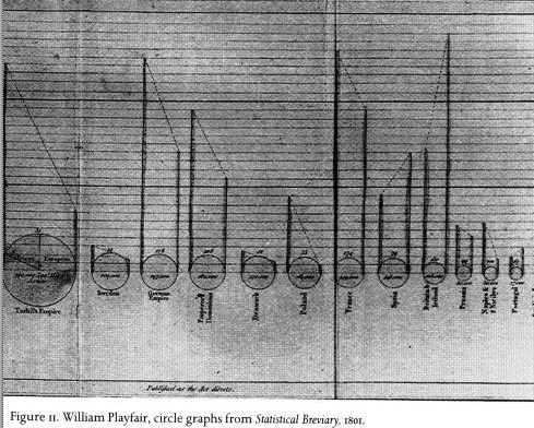
- Data graphics (200 years)
- More abstract, relational views of data (scatterplot, bar chart, pie chart, etc.)
- Visualization (20 years)
- Scientific visualization, modern computer graphics. Low resolution and small
screenspace. Animation, color, and sound.
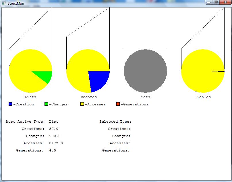
Principles of Graphic Excellence
Graphic designs should tell the truth about a complex situation using
multiple variables. Give viewer the greatest # of ideas, in the shortest
time, using the least "ink", in the smallest space possible.
lecture #35 began here
Ray Tracing
12.1 - Introduction
Ray Tracing is a potentially more accurate form of rendering than the
traditional model provided by OpenGL. Traditionally, it was considered
too slow for real-time, but was fair game in the cinema industry.
Recently, folks such as Intel have announced expectations that next-generation
personal computing platforms will be capable of doing ray-tracing in
real time.
Basic idea: provide a more accurate model of the effect of light in the
rendering. If you start from all the light sources, almost all of your
model effort will be wasted, bouncing light rays on stuff in directions
that won't be visible to the camera. We want to approximate that, with
a shortcut that computes the visible portion of the overall lighting in
the scene.
Idea: "shoot" a ray in reverse from the eye out through each pixel.
The color we see for that pixel will go back to whatever light source
would bounce off something into our field of vision. This is
sort of the opposite of the usual 3D projection-onto-viewport.
Idea: use a parametric equation for the light ray, to walk backwards
into the scene, trying to map it back to a light source after bouncing
off whatever object it hits.
Idea: how far backwards we are willing to trace the ray should depend
on the material surface(s) it hits. Diffuse ones had better be direct
hits from some light source, while shiny ones would reflect, and
transparent ones would refract.
12.2 - Geometry of Ray Tracing
Lots of parameters; overwhelming until familiar. Since Dr. J is a
simpleton, he likes
r(t) = E + Drc * t
E is the eye point (x,y,z), D is the direction vector.
Note that this is not exactly the camera direction, it is the direction
of the eye looking through pixel (r,c), which is non-trivial to compute,
but between your geometry skills and the materials in chapters 6,7 and 12
I expect you could find it.
12.3 - Overview of Ray Tracing
define objects and light sources
set up the camera
for(int r=0; r < nRows; r++)
   for(int c=0; c < nCols; c++) {
      build the rc-th ray
      find ALL intersections of the rcth ray
        with the objects in the scene
      identify the intersection closest to eye
      compute the hit point and normal
        where ray hits object
      find the color of the light eye receives
        long the ray
   }
12.4 Intersection of a Ray with an Object
Use Implicit Form for each shape. Example (sphere):
F(x,y,z) = x2 + y2 + z2 - 1 = 0
Cylinder:
F(x,y,z) = x2 + y2 - 1 = 0 for 0 < z < 1
Intersection will occur at: F(r(t))=0, i.e. solve for
F(E + D * t) = 0
lecture #36 began here
Intersection with a generic (x-y) plane.
Where does F(E + D * t)
cross the z=0 plane? When Ez + Dz * th = 0, i.e. when
- Ez = Dz * thit,
thit = - (Ez / Dz).
Practice exercise: where does ray r(t)=(4,1,3)+(-3,-5,-3)t hit the generic
plane? Ez = 3, Dz=-3, thit = 1.
Intersection with a generic sphere.
Do the substitution and compute thit.
Book says there are two points or no points and
derives the equation using the quadratic formula.
The generic sphere implicit function was F(x,y,z)=x2+y2+z2-1.
Since the distance of the point from the origin is sqrt(x2+y2+z2),
F(x,y,z) = F(P) = |P|2-1.
Substituting (E+Dt) for P, we get
|(E+Dt)|2-1 = |E|2 + 2 (E • Dt) + |Dt|2 - 1 = 0.
Distributing squares and switching terms around we get
(|D|2)t2 + (2 (E • D))t + (|E|2-1) = 0.
As gross as this is, it is a quadratic equation At2 + Bt + C = 0,
where
A=|D|2, B=2(E•D), C=(|E|2-1), so
t = (-(2E•D) ± sqrt((2E•D)2 - 4|D|2|E|2-1 ) / 2 * |D|2
Example exercise: where does r(t)=(3,2,3)+(-3,-2,-3)t hit the generic sphere?
Intersection of the ray with transformed objects
If generic object
is transformed by matrix T, just build the inverse transformed ray
T-1(E+dt) and see where it hits the generic object.
12.5 Organizing a Ray Tracer
The interesting classes are not class Ray(ex,ey,ez,dx,dy,dz) but
the classes Intersection(hits[]) and HitInfo(thit, geo_obj, hpt, hnrm, ...).
12.6 Other Primitives
Proper mathematical intersections of the ray on various graphic primitives;
in this book: squares, cones, ... polyhedron dice and meshes just handle
(brute force) each face one at a time.
12.7 Shading in Ray Tracing
This long section has a lot of ideas for gradually increasing
accuracy of the light model. It is beyond the scope of this course,
but it does mention that, for multiple light sources, you'd be
summing the effects of the light reaching each point. Does
k light sources mean k rays?
Miscellany and Bonus Material
Interactive Curve Example
Let's look at curve.c. This is a
Bezier curve demo of the Evaluators stuff we mentioned a bit ago.
p
Other Curves
Actually, we can play with the polynomials and draw different kinds of
curves.
There were a few class periods devoted to examples, in particular, there were
texture and lighting examples. We grabbed a chainmail texture off a random image
in a random website, converted it into a PPM and read the PPM and used it in an
OpenGL program. And we looked at the "lighting lab" example, which also demonstrated
several materials. We looked at a student example which moved the camera point
(eye position) and played with orthographic versus perspective projection.